Getting Started

Beyond One-Hot. 17 Ways of Transforming Categorical Features Into Numeric Features

All the encodings that are worth knowing — from OrdinalEncoder to CatBoostEncoder — explained and coded from scratch in Python

“Which gradient boostings do you know?”

“Xgboost, LightGBM, Catboost, HistGradient.”

“And which categorical encodings do you know?”

“One-hot.”

I wouldn’t be surprised to hear such a conversation during a data science interview. Still, it would be quite striking, since just a small portion of data-science projects involve machine learning, whereas practically all of them involve some categorical data.

Categorical encoding is the process of transforming a categorical column into one (or more) numeric column(s).

This is necessary because computers are more at ease working with numbers than with strings. Why is that? Because with numbers it’s easy to find relations (such as “bigger”, “smaller”, “double”, “half”). Whereas — when given strings— a computer can say pretty much only whether they are “equal” or “different”.

However, despite its impact, categorical encoding is easily overlooked by data science practitioners.

Categorical encoding is a surprisingly underrated topic.

This why I decided to deepen my knowledge of encoding algorithms. I started from a Python library called “category_encoders” (this is the Github link). Using it is as easy as:

!pip install category_encoders

import category_encoders as ce

ce.OrdinalEncoder().fit_transform(x)

This post is a walkthrough of the 17 encoding algorithms contained in the library . For each algorithm, I provide a short explanation and a Python implementation in few lines of code. The purpose is not to reinvent the wheel, but to realize how the algorithms work under the hood. After all,

“You don’t understand it, until you can code it”.

Not All Encodings Are Created Equal

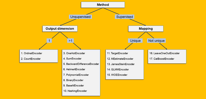
I have classified the 17 encoding algorithms based on some of their characteristics. And since data scientists love decision trees, let’s make them happy:

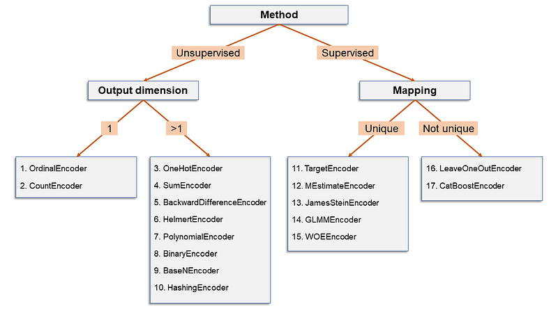
Here’s what the splits refer to:

• Supervised/Unsupervised: when the encoding is based solely on the categorical column, then it’s unsupervised. Otherwise, if the encoding is based on some function of the original column and a second (numeric) column, then it’s supervised.
• Output dimension: the encoding of a categorical column may produce one numeric column (output dimension = 1) or many numeric columns (output dimension > 1).
• Mapping: if each level has always the same output — whether a scalar (e.g. OrdinalEncoder) or an array (e.g. OneHotEncoder)— then the mapping is unique. On the contrary, if the same level is “allowed” to have different possible outputs, then the mapping is not unique.

17 Categorical Encoding Algorithms in 10 Minutes

1. OrdinalEncoder

Each level is mapped to an integer, from 1 to L (where L is the number of levels). In this case we have used alphabetical order, but any other custom order is acceptable.

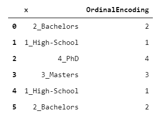
You may think that ordinal encoding is non-sense, especially if the levels have no intrinsic order. You are right! In fact, it’s only a representation of convenience, used often to save memory, or as intermediate step for other types of encoding.

2. CountEncoder

Each level is mapped to the number of observations carrying that level.

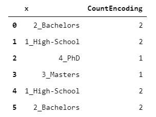
This encoding may be useful as an indicator of the “credibility” of each level. For instance, a machine learning algorithm may automatically decide to take into account the information brought by the level only its count is above some threshold.

3. OneHotEncoder

The encoding algorithm for excellence (and the most used). Each level is mapped to a dummy column (i.e. a column of 0/1), indicating whether that level is carried by that row.

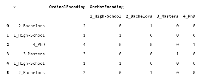
This implies that, whereas your input is a single column, your output consists of L columns (one for each level of the original column). This is why one-hot encoding should be handled with care: you may end up with a dataframe that is far bigger than the original one.

Once the data is one-hot encoded, it’s ready for any predictive algorithm. To make things understandable at first sight, let’s take one observation for each level. Suppose we have observed a target variable, called y, containing the income of each individual (in thousands of dollars). Let’s fit a linear regression (OLS) on the data.

To make the results easily readable, I have attached the OLS coefficients at the side of the table.

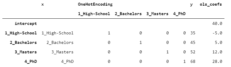
In the case of one-hot encoding, the intercept has no particular meaning, and the coefficients are added to the intercept to obtain the estimate. In this case, since we have just one observation per level, by adding the intercept and the coefficient we obtain the exact value of y (there is no error).

4. SumEncoder

The code that follows may seem a little obscure at first. But don’t worry: in this case, it’s not so important to understand how the encoding is obtained, but how to use it.

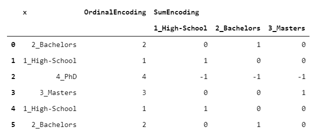
SumEncoder (as the next 3 encoders) belongs to a class called “contrast encodings”. These encodings are designed to have a specific behaviour when used in regression problems. In other words, you use one of these encodings if you want the regression coefficients to have some specific properties.

In particular, SumEncoder is used when you want the regression coefficients to have zero-sum. If we take the same data that we have used in the paragraph above and fit a OLS, this is what we get:

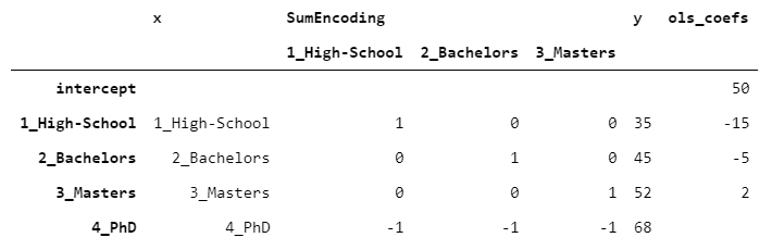
This time, the intercept corresponds to the mean of y. Moreover, by taking y of the last level and subtracting it from the intercept (68-50) we get 18, which is exactly the opposite of the sum of the remaining coefficients (-15-5+2=-18). This is precisely the property of sum encoding that I have mentioned above.

5. BackwardDifferenceEncoder

Another contrast encoding (like SumEncoder).

This encoder is useful for ordinal variables, i.e. variables whose levels can be ordered in a meaningful way. BackwardDifferenceEncoder is designed to compare adjacent levels.

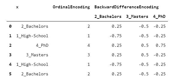
Suppose you have an ordinable variable (e.g. education level) and you want to know how it is related to a numeric variable (e.g. income). It may be interesting to compare each couple of consecutive levels (e.g. bachelors vs. high-school, masters vs. bachelors) with respect to the target variable. This is what BackwardDifferenceEncoder is designed for. Let’s see an example with the same data from the paragraphs above.

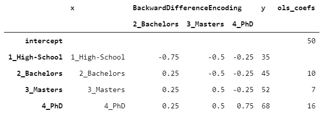
The intercept coincides with the mean of y. The coefficient of Bachelors is 10, because y of Bachelors is 10 higher than High-School, Masters’ coefficient equals 7 because y of Masters is 7 higher than Bachelors and so on.

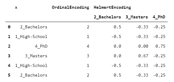
6. HelmertEncoder

HelmertEncoder is very similar to BackwardDifferenceEncoder, but instead of being compared just to the previous one, each level is compared with all the previous levels.

Let’s see what we would get from a OLS model:

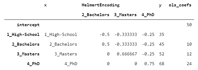
PhD’s coefficient is 24, because PhD is 24 higher than the mean of the previous levels 68-((35+45+52)/3)=24. The same reasoning applies to all the levels.

7. PolynomialEncoder

Another contrast encoding.

As its name suggests, PolynomialEncoder is designed to quantify linear, quadratic and cubic behaviors of the target variable with respect to the categorical variable.

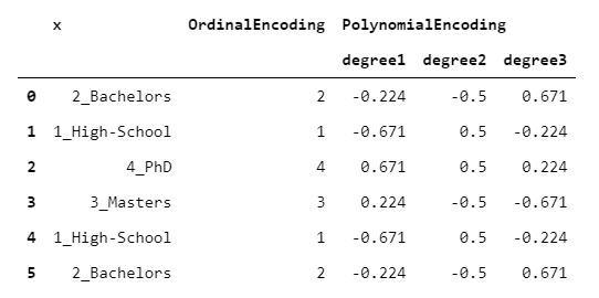
I know what you are thinking. How can a numeric variable have a linear (or quadratic, or cubic) relation with a variable that is not numeric? This is based on the assumption that the underlying categorical variable has levels that are not only ordinable, but also equally spaced.

For this reason, I would suggest to use it with care, only when you are sure that the assumption is reasonable.

8. BinaryEncoder

BinaryEncoder is basically the same of OrdinalEncoder, the only difference is that the integers are converted to binary numbers, then every positional digit is one-hot encoded.

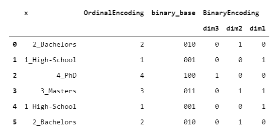
The output consists of dummy columns, as happens for the OneHotEncoder, but it leads to a dimensionality reduction with respect to one-hot.

Honestly, I don’t know any practical application of this type of encoding (if you do, please comment below!).

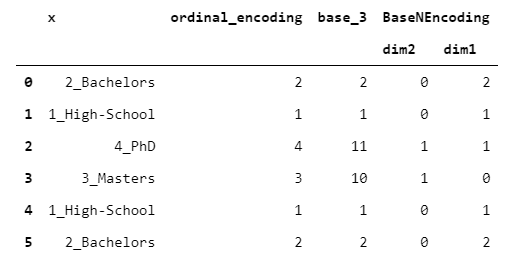
9. BaseNEncoder

BaseNEncoder is simply a generalization of the BinaryEncoder. In fact, in BinaryEncoder, the numbers are in base 2, whereas in BaseNEncoder, numbers are in base n, with n greater than 1.

Let’s see an example with base=3.

Honestly, I don’t know any practical application of this type of encoding (if you do, please comment below!).

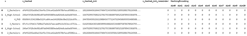
10. HashingEncoder

In HashingEncoder, each original level is hashed, using some hashing algorithm, such as SHA-256. Then, the outcome is converted to integer and the module of that integer with respect to some (big) divisor is taken. By doing so, we have mapped each original string to an integer between 1 and divisor-1. Lastly, the integer that has been obtained by this procedure is one-hot encoded.

Let’s see an example with output_dimension = 10.

The fundamental property of hashing is that the resulting integer is uniformly distributed. So, if you take a divisor big enough, it’s unlikely that two different strings are mapped to the same integer. Why would that be useful? Actually, this has a very practical application called “hashing trick”.

Imagine that you want to make an email spam classifier using a logistic regression. You could do that by one-hot-encoding all the words contained in your dataset. The main downsides are that you would need to store the mapping in a separate dictionary and your model dimensions would change any time that new strings appear.

These issues may be easily overcome by using the hashing trick, because by hashing the input, you don’t need a dictionary anymore and your output dimension is fixed (it depends only on the divisor that you choose initially). Moreover, for the properties of hashing, you are granted that a new string will likely have a different encoding than the existing ones.

11. TargetEncoder

Suppose that you have two variables: one categorical (x) and one numeric (y). Say that you want to transform x into a numeric variable. You may want to employ the information “carried” by y. An obvious idea is to take the mean of y for each level of x. In formula:

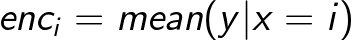
This is reasonable, but there’s a big problem with this approach: some groups may be too small or too variable to be reliable. Many supervised encodings overcome this issue by choosing a middle way between the group mean and the global mean of y:

where w_i is between 0 and 1, depending on how “credible” is the group mean.

The next three algorithms (TargetEncoder, MEstimateEncoder and JamesSteinEncoder) differ based on how they define w_i.

In TargetEncoder, the weight depends on the group numerosity and on a parameter called “smoothing”. When smoothing is 0, we rely solely on group means. Then, as smoothing increases, the global mean weights more and more, leading to a stronger regularization.

Let’s see how the outcome changes with some different values of smoothing.

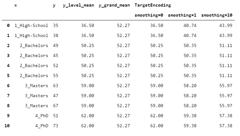
12. MEstimateEncoder

MEstimateEncoder resembles TargetEncoder, but w_i depends on a parameter called “m”, which sets how much the global mean should weight in absolute terms. m is easy to understand because it can be considered as a number of observations: if the level has exactly m observations, then the level mean and the overall mean weight the same.

Let’s see how the outcome changes for different values of m:

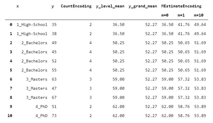
13. JamesSteinEncoder

TargetEncoder and MEstimateEncoder depend both on the group numerosity and on the value of a parameter (respectively smoothing and m) set by the user. This is not convenient, because setting these weights is a manual task.

A natural question is the following: is there a way to set an optimal w_i, without the need of any human intervention? The JamesSteinEncoder tries to do so in a way that is statistically grounded.

The intuition is that the mean of a group with high variance should be trusted less. Therefore, the higher the group variance, the lower the weight (if you want to know more about the formula, I suggest this post by Chris Said).

Let’s see a numeric example:

The JamesSteinEncoder has two significant advantages: it provides better estimates than the maximum-likelihood estimator, and it doesn’t need any parameter setting.

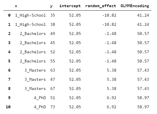
14. GLMMEncoder

GLMMEncoder follows a totally different approach. Basically, it fits a Linear Mixed Effect Model on y. This approach exploits the fact that Linear Mixed Effect Models are designed precisely for handling homogeneous groups of observations (as well explained here). Thus, the idea is to fit a model with no regressors (only the intercept) and to use the levels as groups.

Then, the output is simply the sum of the intercept and the random effect of the group.

15. WOEEncoder

WOEEncoder (which stands for “Weight of Evidence” Encoder) can be employed only for binary target variables, i.e. target variables whose levels are 0/1.

The idea behind Weight of Evidence is that you have two distributions:

• the distribution of 1s (# of 1s in each group / # of 1s in all y)
• the distribution of 0s (# of 0s in each group / # of 0s in all y)

The heart of the algorithm is dividing the distribution of 1s by the distribution of 0s (for each group). Of course, the higher this value, the more confident we are that the group is “skewed” towards 1s, and viceversa. Then, the logarithm of this value is taken.

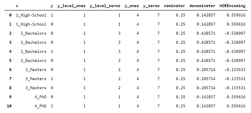
As you can see, due to the presence of a logarithm in the formula, the output is not not directly interpretable. However, it works pretty well as a preprocessing step for machine learning.

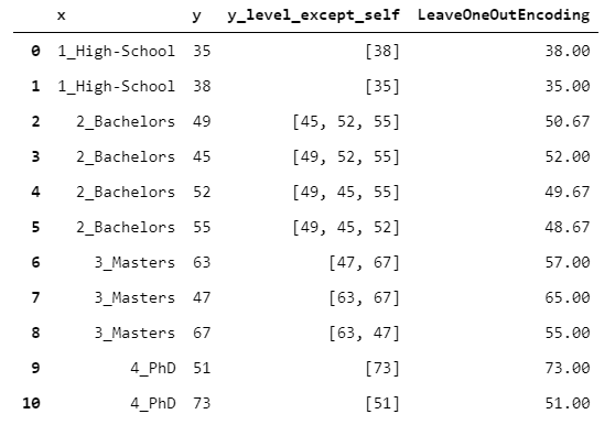
16. LeaveOneOutEncoder

All the 15 encoders seen up until now have a unique mapping.

However, if you plan to use the encoding as input for a predictive model (for example a gradient boosting), this could be a problem. In fact, suppose that you use TargetEncoder. This would imply that you are introducing information about y_train inside X_train, which could lead to a serious risk of overfitting.

The point is: how to maintain a supervised encoding, while limiting the risk of overfitting? LeaveOneOutEncoder offers a brilliant solution. It does a vanilla target encoding but, for each row, it does not consider the value of y observed for that row. In this way, it avoids row-wise leakage.

17. CatBoostEncoder

CatBoost is a gradient boosting algorithm (like XGBoost or LightGBM) that has shown to work extremely well in a wide range of problems. The encoding algorithm is described in detail here (our implementation is a little simplified, but it’s good for grasping the concept).

CatboostEncoder works basically like LeaveOneOutEncoder, but following an on-line approach.

But how to simulate an on-line behaviour in an off-line setting? Imagine that you have a table. Then, take a row somewhere in the middle of the table. What CatBoost does is pretending that the rows above the current row have been observed previously in time, while the rows below have yet to be observed (i.e. will be observed in the future). Then, the algorithm does a leave-one-out encoding, but based only on the rows already observed.

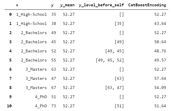
This may seem absurd. Why throwing away some information that could be useful? You can see it simply as more extreme attempt of randomizing the output (i.e. reducing overfitting).

You can find all the code that is in the post (and something more) in this Github notebook.

Thank you for reading!

If you find my work useful, you can subscribe to get an email every time that I publish a new article (usually once a month).

If you want to support my work, you can buy me a coffee.

If you’d like, add me on Linkedin!