Beyond Accuracy: Recall, Precision, F1-Score, ROC-AUC

When talking about classification in Machine Learning, we tend to focus on the test accuracy i.e., how many instances were classified correctly among the total number of test instances. This could be misleading when it comes to imbalanced data. In this post, we will discuss other performance metrics like Recall, Precision, etc., and what additional advantages they offer in comparison to accuracy.

For ease of explanation, let us consider a simple multi-class classification problem with the iris dataset throughout this post. There are three types of flowers setosa, versicolor and virginica which are labelled here as 0, 1, and 2.

Drawbacks of Accuracy

Before discussing other metrics, let us understand the drawbacks of accuracy.

• Let us consider a scenario where 90 samples are from classes versicolor and setosa and only 10 samples of virginica in our sample dataset. The model classifies samples of both the classes correctly and the accuracy is 90%. This might seem high but we miss the 10 misclassified samples of virginica.
• As we are going to see in the subsequent sections, accuracy weighs all kinds of misclassifications equally where as some kinds of errors might be more harmful than the others depending on the situation.

Confusion Matrix

Some of the problems mentioned above can be solved examining measures that are displayed in a confusion matrix. These terms are very intuitive but can be confusing to remember.

True Positives(TP): These are the instances classified correctly i.e., the test instances that have been classified with their true classes.

True Negatives(TN): These are the test instances that belong to the Negative class and have been predicted correctly.

These two can be remembered as it is “True” that these are positive or negative respectively.

Based on the knowledge above, pause and think about what False Positives or False Negatives could be.

False Positives(FP): These are the instances that have been incorrectly classified as Positive but their actual class is Negative.

False Negatives(FN): These are the instances that have been incorrectly classified as Negative but their actual class is Positive.

These two can be remembered as it is “False” that these are positive or negative respectively and hence they indicate incorrect predictions.

With the help of below code taken from GeeksForGeeks, we will fit a Decision Tree Classifier to the iris data and obtain a prediction.

from sklearn import datasets
from sklearn.metrics import confusion_matrix, plot_confusion_matrix
from sklearn.model_selection import train_test_split
import numpy as np
import matplotlib.pyplot as plt
from sklearn.tree import DecisionTreeClassifier

# loading the iris dataset
iris = datasets.load_iris()
X = iris.data
y = iris.target

# dividing X, y into train and test data
X_train, X_test, y_train, y_test = train_test_split(X, y, random_state = 0)

dtree_model = DecisionTreeClassifier(max_depth = 2).fit(X_train, y_train)
plot_confusion_matrix(dtree_model, X_test, y_test)

This is the Confusion matrix from the above code.

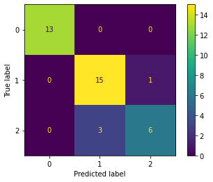
Now, let us label the TP, FP, TN, FN from this matrix. Since there are 3 classes, these values are calculated for each class. The diagonal elements show the correct predictions.

For Class 0, the TPs are 13 i.e., all of them are classified correctly and hence TN = FN = FP = 0. For Class 1, the TP = 15, FN = 1, FP = 3. As an exercise come up with the values for Class 2(TP = 6, FN = 3, FP = 1).

Recall

This is also called Sensitivity. This indicates out of all the instances that actually belong to a class(True Positives + False Negatives), how many were classified correctly. This tells the ability of a model to classify the instances of a particular class correctly.

Recall = True Positives / (True Positives + False Negatives)

Precision

This is also called Positive Predictive Value. This metric measures out of all the instances classified with a particular class(True Positives + False Positives) how many instances actually belong to the class. If our model classifies something as positive, precision indicates how confident we can be that it is actually positive.

Precision = True Positives / (True Positives + False Positives)

Recall vs(and) Precision

In the above example, class 0 has 13 samples and all of them have been classified correctly. Now, let us say along with these 13 samples, 7 instances of class 2 have also been classified as class 0. In this case, we have a recall of 100% but the precision is only 65%. Had we used only recall to evaluate the model it would have been misleading. Hence, we need to examine both for evaluation of our models. Sometimes it also happens that increasing the precision results in decrease of recall and vice-versa.

When a measure is more important may also change based on our use-case. For example, in serious issues like a cancer diagnosis, having False Negatives could be dangerous as people with cancer might go un-treated which results in the disease becoming worse. On the other hand, if someone is classified falsely as positive, more clinical tests can be conducted and they can be assured as healthy. In such cases, we aim for high recall. In the case of finding an accused person guilty, a False Positive(labelling a non-criminal as guilty) might be considered more serious and hence we aim for higher precision.

F1-Score

As Recall and Precision could be at odds, to achieve a balance we could combine them into a single measure known as F1-Score.

F1-score is defined as a harmonic mean of Precision and Recall and like Recall and Precision, it lies between 0 and 1. The closer the value is to 1, the better our model is. The F1-score depends both on Recall and Precision.

F1-Score = 2 * Precision * Recall/(Precision + Recall)

All the above measures for each class can be calculated using sklearn classification report:

print(classification_report(y_test, dtree_predictions, target_names=['class 0', 'class 1', 'class 2']))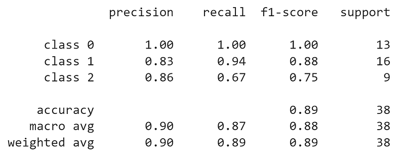

From the above report, we can see that overall accuracy is 0.89 and precision, recall, and f1-score for each class have been calculated. Let us verify the scores for class 1 from our calculations of TP, FP, FN, TN above.

For Class 1, TP = 15, FN = 1, FP = 3
Recall = 15/(15 + 1) = 0.94
Precision = 15/(15 + 3) = 0.83
F1-Score = 2 * 0.94 * 0.83/(0.94 + 0.83) = 0.88

The macro and weighted averages are the average of each of the scores. The macro only takes mean of the measures for the three classes whereas the measures are weighted by the class proportion to get the weighted average. These can be used as the final scores of a model and can be further used for comparison with other models.

ROC-AUC Curve

Another popular way to measure model performance is the ROC-AUC curve/score. Receiver Operating Characteristic Curve shows the performance of the model at different threshold values used for the classification. It plots True Positive Rate on the y-axis and False Positive Rate on the x-axis, that has been calculated at each probability threshold. This curve helps to measure the model’s ability to distinguish between two classes. Like we saw in the previous examples, it is not enough to just have a high recall, we also need to take care that FPs are not too high.

Apart from the recall(sensitivity or True Positive Rate), there are many other metrics that can be calculated from the confusion matrix. One of them is the False Positive Rate which is calculated as follows. This False Positive Rate can also be calculated as 1 — Specificity.

Specificity = True Negatives/(True Negatives + False Positives)

False Positive Rate = Number of False Positives/(Number of False Positives + True Negatives)

In general, our aim is to reduce False Positive Rate and have a high True Positive Rate. In order to measure this, we calculate AUC which stands for Area Under the ROC-Curve. This lies between 0 and 1 and the closer AUC is to 1, the better our model is. If the AUC is zero, all predictions are False Positives and the performance is bad. If AUC is one, the model differentiates between the two classes perfectly and the curve is a horizontal line. If the AUC is 0.5, the TPR and FPR are equal and the model is as good as a random prediction. Usually, AUC score of 0.8 or 0.9 is considered to be good.

The ROC-AUC curve can only used for a binary classification problem. In a multi-classification setting we need to modify the problem into OneVsRestClassification i.e., for plotting the graphs, we first consider Class 0 as the positive class and classes 1 and 2 will be considered the negative class. Similarly, we consider Class 1 as the positive class and classes 0 and 1 as the negative class and this is similar for Class 2. Alternatively, we could also plot the ROC-AUC curve with OneVsOneClassification, and measure the model’s ability to distinguish any two classes by ignoring the third class.

Let us apply the strategy to our current problem using the code given here Scikit-Code-Multi-Class. We change the code to use a decision tree classifier with max_depth = 2 instead of the SVM and plot the ROC-AUC curve of each class.

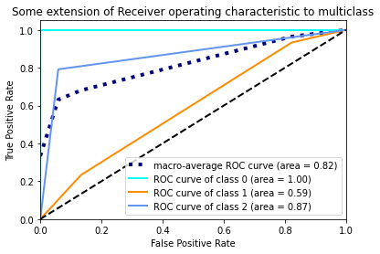
From the above graph, we can see ROC-curves of different classes. The class 0 has the highest AUC and class 1 has the lowest AUC. The black dashed line represents random predictions and the blue one shows the average AUC of all three classes. With this information, we could build better models that improve AUC of class 1 and class 2. Here, the AUC represents how well the model distinguishes a particular class from rest of the classes.

In this post, we have discussed some classification metrics which have formed a basis for more advanced metrics. Understanding them is important in optimization and selection of appropriate models.

References

I am a student of Masters in Data Science @ TU Dortmund. Feel free to connect with me on LinkedIn for any feedback on my posts or any professional communication.