
Bayesian Linear Regression from Scratch in Python: A Comprehensive Guide
Learn how to implement linear regression in Bayesian framework

(This article presume you have a basic knowledge on linear regression, Bayesian inference and MCMC. If you wanna know more about MCMC, please check my previous post shown below.)
1. Introduction
Everyone who is interested in any data-related area must familiar with linear regression. It is the most fundamental and basic regression method that must be covered in every statistics and machine learning courses. Many advanced models are also developed based on linear regression such as generalised linear model (GLM) and polynomial regression.
Traditionally, ordinary least square (OLS) is used to estimate the linear regression coefficients. We can also use maximum likelihood estimates (MLE) when the distribution of the error terms is known. We refer this type of regression as ‘frequentist’ linear regression.
Bayesian linear regression, as its name suggests, is simply the linear regression but implemented under a Bayesian framework, which is a powerful way to integrate our prior knowledge and update beliefs based on observed data. The Bayesian approach gives the estimate of the posterior distribution for the regression coefficients. It provides a range of values for the coefficients, capturing uncertainty more comprehensively than a point estimate.
In this article, I will first have a quick recap on the concept of linear regression, then explain the Bayesian linear regression along with the derivation of its posterior distribution. Lastly, I will demonstrate how to use Gibbs sampler to implement Bayesian linear regression from scratch with Python.
2. Classical linear regression
Linear regression is a statistical method to model the relationship between a dependent variable and a series of independent variables by fitting a linear model to the observed data, where the best-fitting line can be obtained using OLS method. Suppose we have a dependent variable y ∈ℝⁿ and a data matrix X ∈ℝⁿᵖ, the linear model can be written as follow:

where θ is the regression coefficient and ε is the error term. OLS method estimates the regression coefficients by minimising the sum of squared error:

We can use calculus to obtain θ that minimise the loss function. The gradient of ℒ with respect to θ is

Setting ∇ℒ = 0 to obtain the OLS estimate of θ:

If we make the Gaussian assumption on ε, we can estimate θ using MLE, and it will yield the same result as OLS does. Furthermore, with the Gaussian assumption, we can derive the distribution of θ ‘hat’. This allows users to conduct hypothesis tests on the regression coefficients and access the uncertainty of the estimator. The distribution of θ ‘hat’ is

Note that the Gaussian assumption is not necessary to obtain the OLS estimate, but it facilitates statistical inference and hypothesis testing, and simplifies the mathematical derivation of certain properties of the estimators.
3. Bayesian Linear Regression
In Bayesian linear regression, we don’t treat the regression coefficient as a fixed parameter anymore. Instead, we regard it as a random variable, and our goal is to update its distribution based on the data (y, X). With the Gaussian assumption, the linear model can be written as:

where θ and σ² is the model parameters. Just like in other Bayesian problems, we have the freedom to pick priors based on what we know. If our knowledge about θ and σ is a bit fuzzy, we can opt for an informative (or weakly-informative) prior. One handy choice is the conjugate prior, which yield a posterior distribution that mirrors the prior one.

θ₀, Σ, α and β are called hyper-parameters. To estimate the joint posterior with Gibbs sampler, we compute the conditional posterior f(θ | σ², y, X) and f(σ² | θ, y, X) respectively. The conditional posterior of θ is

The posterior distribution of σ² is

Do they look tedious? Rewrite the posterior:

4. Gibbs sampler
The Gibbs sampler is one of the MCMC methods used to draw samples from a multivariate distribution. It is particularly useful when direct sampling from a joint distribution is challenging, but sampling from its conditional distributions is straightforward.
In our case, f(θ | σ², y, X) follows a multivariate normal distribution, and f(σ² | θ, y, X) follows an inverse-gamma distribution. These distributions are well-known, and direct sampling with them is really simple. Therefore, we will use the Gibbs sampler to estimate the posterior.
The algorithm of the Gibbs sampler is:
- Initialise θ₀ and σ₀
- For each iteration i, do
- Sample θᵢ ~ f( . | σᵢ₋₁)
- Sample σᵢ ~ f( . | θᵢ)
Notice that we use the most-updated values of θ and σ for sampling. We sample σᵢ from f(σ² | θᵢ, y, X) but not f(σ² | θᵢ₋₁, y, X) because we already have the value of θᵢ.
5. Coding Part
In this article, I will use abalone dataset to demonstrate how to perform Bayesian linear regression from scratch in Python (only some basic libraries like numpy, pandas and matplotlib will be used). I will also use statsmodels to compare the results between the frequentist approach and the bayesian approach.
5.1. Import libraries and clean abalone dataset
First we need to import the required libraries and load the dataset. The abalone dataset can be obtained at UCI Machine Learning Repository.
import numpy as np
from numpy.linalg import inv

import pandas as pd
import matplotlib.pyplot as plt

from ucimlrepo import fetch_ucirepo

# fetch dataset
abalone = fetch_ucirepo(id=1)

# data (as pandas dataframes)
X = abalone.data.features
y = abalone.data.targets

# show first 5 rows
X.head()

##        | Sex | Length | Diameter | Height | Whole_weight | Shucked_weight  | Viscera_weight | Shell_weight |
## -------|-----|--------|----------|--------|--------------|-----------------|----------------|--------------|
##    0   |  M  | 0.455  |  0.365   | 0.095  |    0.5140    |     0.2245      |     0.1010     |    0.1500    |
##    1   |  M  | 0.350  |  0.265   | 0.090  |    0.2255    |     0.0995      |     0.0485     |    0.0700    |
##    2   |  F  | 0.530  |  0.420   | 0.135  |    0.6770    |     0.2565      |     0.1415     |    0.2100    |
##    3   |  M  | 0.440  |  0.365   | 0.125  |    0.5160    |     0.2155      |     0.1140     |    0.1550    |
##    4   |  I  | 0.330  |  0.255   | 0.080  |    0.2050    |     0.0895      |     0.0395     |    0.0550    |
You may notice that there is an ‘I’ in the fifth row of Sex. According to the abalone’s variables table, ‘I’ stands for infant abalones. It represents that the abalones are in the early stage of development and have not yet reached sexual maturity. Let’s check its frequency distribution and consider excluding rows corresponding to infant abalones in cases where there are only a few records of them.
# get the distribution of abalones by Sex
fig, ax = plt.subplots(figsize=(5,3))
ax.bar(X['Sex'].value_counts().index, X['Sex'].value_counts())
ax.set_xticklabels(['Male', 'Infant', 'Female'])
ax.set_ylabel('Count')
ax.set_title('Sex Distribution of Abalones')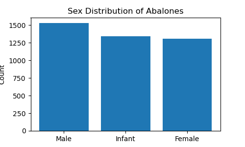
It shows that there is a substantial number of male, infant and female abalones, with a relatively even distribution among the three categories. We will keep the infant abalones’ records and one-hot encode the Sex column.
# one-hot encode Sex column
abalone_sex = pd.get_dummies(X['Sex'])
abalone_sex = abalone_sex.drop(columns='I')
abalone_sex = abalone_sex.astype(int)
abalone_sex.columns = ['IsFemale', 'IsMale']
X = pd.concat([abalone_sex, X], axis=1)

# add intercept column
X['Intercept'] = 1
X = X[['Intercept'] + [col for col in X.columns if col not in ['Intercept', 'Sex']]]
X.head()

##        | Intercept | IsFemale | IsMale | Length | Diameter | Height | Whole_weight | Shucked_weight  | Viscera_weight | Shell_weight |
## -------|-----------|----------|--------|--------|----------|--------|--------------|-----------------|----------------|--------------|
##    0   |     1     |    0     |   1    | 0.455  |  0.365   | 0.095  |    0.5140    |     0.2245      |     0.1010     |    0.1500    |
##    1   |     1     |    0     |   1    | 0.350  |  0.265   | 0.090  |    0.2255    |     0.0995      |     0.0485     |    0.0700    |
##    2   |     1     |    1     |   0    | 0.530  |  0.420   | 0.135  |    0.6770    |     0.2565      |     0.1415     |    0.2100    |
##    3   |     1     |    0     |   1    | 0.440  |  0.365   | 0.125  |    0.5160    |     0.2155      |     0.1140     |    0.1550    |
##    4   |     1     |    0     |   0    | 0.330  |  0.255   | 0.080  |    0.2050    |     0.0895      |     0.0395     |    0.0550    |
We also added the intercept column which has all entries equal to 1. Our dataset now is ready. Let’s see how to perform Bayesian linear regression.
5.2. Estimate posterior distribution of θ and σ² with Gibbs
I created a class BayesianLinearRegression that contains several useful methods for fitting Bayesian linear model and diagnosing the MCMC samples.
class BayesianLinearRegression:

    def __init__(self, nIter=2**12, pBurn=None):
        self.nIter = nIter
        self.pBurn = pBurn if pBurn is not None else 0.5

    def fit(self, y, X, theta0=None, Sigma=None, alpha=None, beta=None):

        self.colnames = X.columns

        if isinstance(y, pd.Series):
            y = y.to_numpy()
        if isinstance(X, pd.DataFrame):
            X = X.to_numpy()

        self.n, self.p = X.shape
        self.theta0 = theta0 if theta0 is not None else np.zeros(self.p)
        self.Sigma = Sigma if Sigma is not None else np.diag(np.ones(self.p))
        self.alpha = alpha if alpha is not None else 1
        self.beta = beta if beta is not None else 1
        theta = np.empty((self.nIter+1, self.p))
        sigma2 = np.empty(self.nIter+1)
        theta[0] = np.random.normal(size=self.p)
        sigma2[0] = np.random.exponential(size=1)

        for iIter in range(1, self.nIter+1, 1):
            # update theta
            inv_Sigma = inv(self.Sigma)
            inv_comp1 = inv(np.matmul(X.T, X)/sigma2[iIter-1] + inv_Sigma)
            comp2 = np.matmul(X.T, y)/sigma2[iIter-1] + np.matmul(inv_Sigma, self.theta0)
            theta[iIter] = np.random.multivariate_normal(np.matmul(inv_comp1, comp2), inv_comp1, 1)
            # update sigma2
            e = y - np.matmul(X, theta[iIter])
            alpha_n = self.alpha + self.n/2
            beta_n = self.beta + np.matmul(e.T, e)/2
            sigma2[iIter] = 1/np.random.gamma(alpha_n, 1/beta_n, 1)

        self.thetaAll = pd.DataFrame(theta, columns=self.colnames)
        self.sigma2All = pd.DataFrame(sigma2, columns=['sigma2'])
        self.thetaBurn, self.theta = self._burn(self.thetaAll)
        self.sigma2Burn, self.sigma2 = self._burn(self.sigma2All)

    def _burn(self, theta):
        self.nBurn = int(self.nIter * self.pBurn)
        return theta.iloc[:self.nBurn,:], theta.iloc[self.nBurn:,:]

    def get_credible_interval(self):
        index_labels = ['2.5%', '50%', '97.5%']
        theta_ci = np.quantile(self.theta, [0.025, 0.5, 0.975], axis=0)
        sigma2_ci = np.quantile(self.sigma2, [0.025, 0.5, 0.975]).reshape((3,1))
        self.theta_ci = pd.DataFrame(theta_ci, columns=self.colnames, index=index_labels)
        self.sigma2_ci = pd.DataFrame(sigma2_ci, columns=['sigma2'], index=index_labels)

    def plot_posterior(self, variables='all'):

        self.get_credible_interval()

        if variables=='all':
            n_vars = self.p
            variables = self.colnames

        n_vars = len(variables) + 1
        n_fcols = int(np.ceil(np.sqrt(n_vars)))
        n_frows = int(np.ceil(n_vars/n_fcols))
        fig, axs = plt.subplots(n_frows, n_fcols, figsize=(4*n_fcols, 4*n_frows), squeeze=False)
        self.sigma2.plot(kind='kde', ax=axs[0,0], label=r'$f(\sigma^2\mid\mathrm{y},\mathrm{X})$')
        axs[0,0].axvline(self.sigma2_ci.loc['50%', 'sigma2'], color='red', linestyle='dashed', linewidth=2, label=r'$\widehat{\sigma}^2$')
        axs[0,0].set_title(r'$\sigma^2$')
        axs[0,0].legend(loc='upper right')

        i, j = 0, 1
        for col in variables:
            self.theta[col].plot(kind='kde', ax=axs[i,j], label=r'$f(\theta\mid\mathrm{y},\mathrm{X})$')
            axs[i,j].axvline(self.theta_ci.loc['50%', col], color='red', linestyle='dashed', linewidth=2, label=r'$\widehat{\theta}$')
            axs[i,j].set_title(col)
            axs[i,j].legend(loc='upper right')
            j += 1
            if j % n_fcols == 0:
                j = 0
                i += 1

    def trace_plot(self, first_n=200):

        fig, axs = plt.subplots(1, 2, squeeze=False, figsize=(5*2, 3))

        # First n=200 samples
        thetaFirst200 = self.thetaBurn.iloc[0:first_n,:]
        sigma2First200 = self.sigma2Burn.iloc[0:first_n,:]
        axs[0,0].plot(sigma2First200.index, sigma2First200['sigma2'], label=r'$\sigma^2$', linestyle='-')
        for col in thetaFirst200.columns:
            axs[0,0].plot(thetaFirst200.index, thetaFirst200[col], label=col, linestyle='-')
        axs[0,0].set_xlabel('Index')
        axs[0,0].set_ylabel('Value')
        axs[0,0].set_title('Trace plot of ' + r'$\theta_{1:%s}$' % first_n)
        axs[0,0].grid(True)

        # Latter part of the Markov-chain
        axs[0,1].plot(self.sigma2.index, self.sigma2['sigma2'], label=r'$\sigma^2$', linestyle='-')
        for col in self.theta.columns:
            axs[0,1].plot(self.theta.index, self.theta[col], label=col, linestyle='-')
        axs[0,1].set_xlabel('Index')
        axs[0,1].set_ylabel('Value')
        axs[0,1].set_title('Trace plot of $\\theta_{{{}:{}}}$'.format(self.theta.index[0], self.theta.index[-1]))
        axs[0,1].legend(bbox_to_anchor=(1, 0.5), loc='center left')
        axs[0,1].grid(True)

    def acf_plot(self):

        n_vars = self.p + 1
        n_fcols = int(np.ceil(np.sqrt(n_vars)))
        n_frows = int(np.ceil(n_vars/n_fcols))
        fig, axs = plt.subplots(n_frows, n_fcols, figsize=(4*n_fcols, 4*n_frows), squeeze=False)
        plot_acf(self.sigma2All['sigma2'], lags=20, ax=axs[0,0])
        axs[0,0].set_title(r'$\sigma^2$')
        axs[0,0].set_ylim([-0.1, 1.1])

        i, j = 0, 1
        for col in self.thetaAll.columns:
            plot_acf(self.thetaAll[col], lags=20, ax=axs[i,j])
            axs[i,j].set_title(col)
            axs[i,j].set_ylim([-0.1, 1.1])
            j += 1
            if j % n_fcols == 0:
                j = 0
                i += 1
Methods of BayesianLinearRegression :
fit: fit Bayesian linear model to the dataset_burn: burn-in Markov chainget_credible_interval: return 95% credible interval of θ and σ²plot_posterior: plot the kernel density estimator (KDE) for θ and σ²trace_plot: get the trace plot of first 200 Markov chain and the trace plot of the used samplesacf_plot: plot the autocorrelation (ACF) for θ and σ²
y = y['Rings']
nIter = 2**14
pBurn = 0.5
model = BayesianLinearRegression(nIter, pBurn)
model.fit(y, X)
To get the Bayes estimator under L₁-loss and 95% credible interval for θ and σ²:
model.get_credible_interval()
print(model.theta_ci)

##          | Intercept | IsFemale | IsMale | Length | Diameter | Height | Whole_weight | Shucked_weight  | Viscera_weight  | Shell_weight |
## ---------|-----------|----------|--------|--------|----------|--------|--------------|-----------------|-----------------|--------------|
##   2.5%   | 3.2915    | 0.8010   | 0.7991 | 2.2293 | 3.3068   | 2.8143 | 3.9159       | -14.3075        | -4.6137         | 8.7121       |
##   50%    | 3.7318    | 0.9989   | 0.9850 | 3.6405 | 4.9242   | 4.4861 | 4.7185       | -13.2287        | -3.1100         | 10.0295      |
##   97.5%  | 4.1679    | 1.2009   | 1.1711 | 5.0367 | 6.5046   | 6.1138 | 5.5016       | -12.1086        | -1.5382         | 11.3662      |

print(model.sigma2_ci)

##          | sigma2   |
## ---------|----------|
##   2.5%   | 4.7825   |
##   50%    | 4.9989   |
##   97.5%  | 5.2170   |
For the classical linear regression, we can use statsmodels to get the OLS estimator.
ols_result = sm.OLS(y, X).fit()
print(ols_result.params)

## Intercept          3.069765
## IsFemale           0.824876
## IsMale             0.882592
## Length            -0.458335
## Diameter          11.075103
## Height            10.761537
## Whole_weight       8.975445
## Shucked_weight   -19.786867
## Viscera_weight   -10.581827
## Shell_weight       8.741806
## dtype: float64
It is clear that there are some differences between these two methods. Only the Bayes estimator and OLS estimator for Intercept, IsFemale and IsMale are consistent. For other variables, both methods give a slightly different results.
5.3. Diagnose Markov chain
Use plot_posterior to check the shape for each θ and σ².
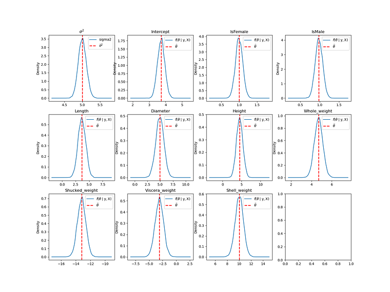
The above graph shows the density estimate for each θ and σ². The blue curve is the KDE and the red dotted vertical line is the posterior median. We can see that the shape for each θ and σ² are also Gaussian.
Use trace_plot to check the value of θ and σ² for each iteration.
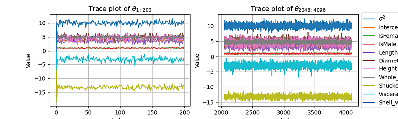
This is the trace plot of the Markov chain. We can see that the Markov chain converges to the target distribution very quickly, reaching convergence after only a few iterations.
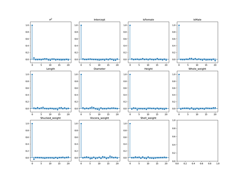
Use acf_plot to check the autocorrelation.
6. Conclusion
This article covers most of the essential knowledge to guide you how to write your own Bayesian linear regression from scratch in Python. It’s always good to code from scratch when you start learning a new model, as it ensures that you can completely understand the underlying concepts. In the future, I will introduce more Bayesian regression related topics such as BIC and LASSO. I will also explain the Gibbs samplers in details.
If you’d like to stay connected, please follow me on Medium 📖.
If you found this article useful, please don’t forget to give it a clap 👏.
Feel free to share your thoughts in the comments — I love hearing from you!