Marketing Analytics

Bayesian Hierarchical Marketing Mix Modeling in PyMC

Learn how to build MMMs for different countries the right way

Imagine that you work in a marketing department and want to investigate if your advertising investments paid off. People who read my other articles know how to do this: marketing mix modeling! This method is fascinating because it also works in a cookieless world.

I have also covered Bayesian marketing mix modeling, a way to get more robust models and uncertainty estimates for everything you forecast.

The Bayesian approach works exceptionally well for homogeneous data, meaning that the effects of your advertising spendings are comparable across your dataset. But what happens when we have a heterogeneous dataset, for example, spendings across several countries? Two obvious ways to deal with it are the following:

1. Ignore the fact that there are several countries in the dataset and build a single big model.
2. Build one model per country.

Unfortunately, both methods have their disadvantages. Long story short: Ignoring the country leaves you with a too-coarse model; probably, it will be underfitting. On the other hand, if you build a model per country, you might end up with too many models to keep track of. And even worse, if some countries don’t have many data points, your model there might overfit.

Usually, it is more efficient to create a hybrid model that is somewhat between these two approaches: Bayesian hierarchical modeling! You can read more about it here as well:

How can we benefit from this in our case exactly, you ask? For example, Bayesian hierarchical modeling could produce a model where the TV carryover values in neighboring countries are not too far apart, which counters overfitting effects.

However, if the data suggests that parameters are, in fact, completely different, the Bayesian hierarchical model will be able to pick this up as well, given enough data.

In the following, I will show you how to combine the Bayesian marketing mix modeling (BMMM) with the Bayesian hierarchical modeling (BHM) approach to create a — maybe you guessed it — a Bayesian hierarchical marketing mix model (BHMMM) in Python using PyMC.

BHMMM = BMMM + BHM

Researchers from the former Google Inc. have also written a paper about this idea that I encourage you to check out later as well. [1] You should be able to understand this paper quite well after you have understood my articles about BMMM and BHM.

Note that I do not use PyMC3 anymore but PyMC, which is a facelift of this great library. Fortunately, if you knew PyMC3 before, you can also pick up on PyMC. Let’s get started!

Preparations

First, we will load a synthetic dataset I made up, which is acceptable for training purposes.

dataset_link = "https://raw.githubusercontent.com/Garve/datasets/fdb81840fb96faeda5a874efa1b9bbfb83ce1929/bhmmm.csv"

data = pd.read_csv(dataset_link)

X = data.drop(columns=["Sales", "Date"])
y = data["Sales"]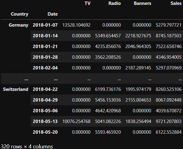

Now, let me copy over some functions from my other article, one for computing exponential saturation and one for dealing with carryovers. I adjusted them — i.e., I changed theano.tensor to aesara.tensor, and tt to at — to work with the new PyMC.

import aesara.tensor as at

def saturate(x, a):
    return 1 - at.exp(-a*x)

def carryover(x, strength, length=21):
    w = at.as_tensor_variable(
        [at.power(strength, i) for i in range(length)]
    )
    
    x_lags = at.stack(
        [at.concatenate([
            at.zeros(i),
            x[:x.shape[0]-i]
        ]) for i in range(length)]
    )
    
    return at.dot(w, x_lags)

We can start modeling now.

BHMMM Building

Before starting with the full model, we could start by building separate models just to see what happens and to have a baseline.

Separate Models

If we follow the methodology from here, we get the following for Germany:

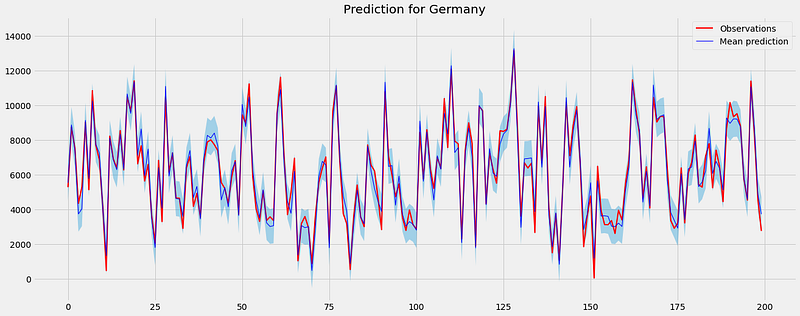
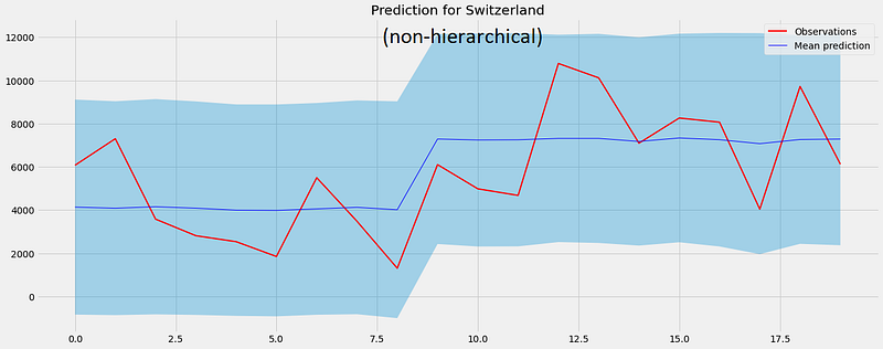
Quite an excellent fit. However, for Switzerland, we only have 20 observations, so the predictions are not too great:

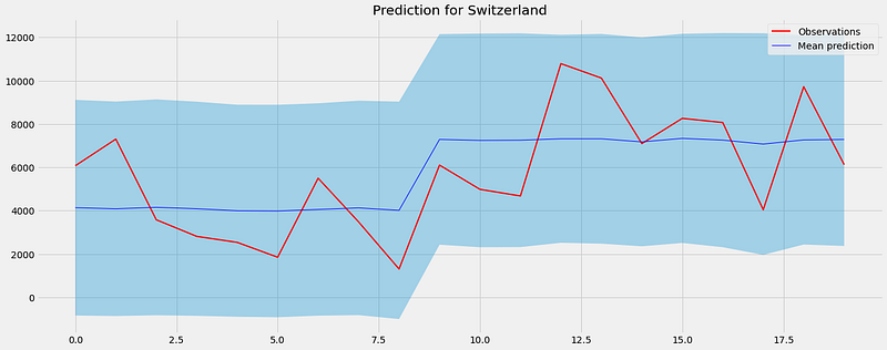
This is precisely the reason why the separate models approach is sometimes problematic. There is reason to believe that the people in Switzerland are not entirely different from those in Germany regarding the impact of media on them, and a model should be able to capture this.

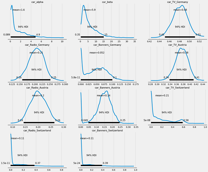
We can also see what the Switzerland model has learned about the parameters:

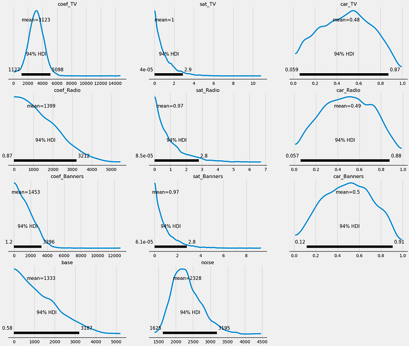
The posteriors are still quite wide due to the lack of Switzerland data points. You can see this from the car_ parameters on the right: the 94% HDI of the carryovers nearly spans across the entire possible range between 0 and 1.

Let us build a proper BHMMM now so especially Switzerland can benefit from the larger amount of data that we have from Germany and Austria.

PyMC Implementation

We introduce some hyperpriors that shape the underlying distribution over all countries. For example, the carryover is modeled using a Beta distribution. This distribution has two parameters α and β, and we reserve two hyperpriors car_alpha and car_beta to model these.

In Line 15, you can see how the hyperpriors are used then to define the carryover per country and channel. Furthermore, I use more tuning steps than usual — 3000 instead of 1000 — because the model is quite complex. Having more tuning steps gives the model an easier time inferring.

with pm.Model() as bhmmm:
    # Hyperpriors
    coef_lam = pm.Exponential("coef_lam", lam=10)
    sat_lam = pm.Exponential("sat_lam", lam=10)
    car_alpha = pm.Exponential("car_alpha", lam=0.01)
    car_beta = pm.Exponential("car_beta", lam=0.01)
    base_lam = pm.Exponential("base_lam", lam=10)

    # For each country
    for country in X["Country"].unique():
        X_ = X[X["Country"] == country]
        channel_contributions = []

        # For each channel, like in the case without hierarchies
        for channel in ["TV", "Radio", "Banners"]:
            coef = pm.Exponential(f"coef_{channel}_{country}", lam=coef_lam)
            sat = pm.Exponential(f"sat_{channel}_{country}", lam=sat_lam)
            car = pm.Beta(f"car_{channel}_{country}", alpha=car_alpha, beta=car_beta)

            channel_data = X_[channel].values
            channel_contribution = pm.Deterministic(
                f"contribution_{channel}_{country}",
                coef * saturate(carryover(channel_data, car), sat),
            )

            channel_contributions.append(channel_contribution)

        base = pm.Exponential(f"base_{country}", lam=base_lam)
        noise = pm.Exponential(f"noise_{country}", lam=0.001)

        sales = pm.Normal(
            f"sales_{country}",
            mu=sum(channel_contributions) + base,
            sigma=noise,
            observed=y[X_.index].values,
        )

    trace = pm.sample(tune=3000)

And that’s it!

Checking the Output

Let us only examine how well the model captures the data.

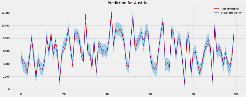
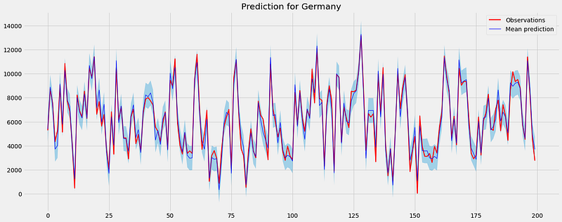
I will not conduct any real checks with metrics now, but from the plots, we can see that the performance of Germany and Austria looks quite well.

If we compare Switzerland from the BHMMM to the version of the BMMM from before, we can also see that it looks so much better now.

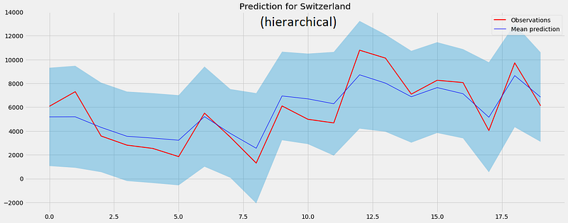
This is only possible because we have given Switzerland some context using the data of other similar countries.

We can also see how the posteriors of the carryovers of Switzerland narrowed down:

Some distributions are still a bit wild, and we would have to look deeper into how to fix this. There might be sampling issues, or the priors might be bad, among other things. However, we will not do that here.

Conclusion

In this article, we have taken a quick look at two different Bayesian concepts:

• Bayesian marketing mix modeling to analyze marketing spendings, as well as
• Bayesian hierarchical modeling.

Combining both approaches, we forged an even better Bayesian marketing mix model. This is especially handy if you deal with some hierarchy, for example, when building a marketing mix model for several related countries.

This method works so well because it gives the model context: if you tell the model to provide a forecast for one country, it can take the information about other countries into account. This is crucial if the model has to operate on an otherwise too-small dataset.

Another thought I want to give you on your way is the following: In this article, we used a country hierarchy. However, you can also think of other hierarchies, for example, a channel hierarchy. A channel hierarchy can arise if you say that different channels should behave not too differently, for instance, if your model not only takes banner spendings but banner spendings on website A and banner spendings on website B, where the user behavior of websites A and B are not too different.

References

[1] Y. Sun, Y. Wang, Y. Jin, D. Chan, J. Koehler, Geo-level Bayesian Hierarchical Media Mix Modeling (2017)

I hope that you learned something new, interesting, and useful today. Thanks for reading!

If you have any questions, write me on LinkedIn!

And if you want to dive deeper into the world of algorithms, give my new publication All About Algorithms a try! I’m still searching for writers!