
Basics of Reinforcement Learning, the Easy Way

Update: The best way of learning and practicing Reinforcement Learning is by going to http://rl-lab.com
Reinforcement Learning (RL) is the problem of studying an agent in an environment, the agent has to interact with the environment in order to maximize some cumulative rewards.
Example of RL is an agent in a labyrinth trying to find its way out. The fastest it can find the exit, the better reward it will get.

Markov Decision Process (MDP)
To describe this problem in a mathematical way, we use Markov Decision Process (MDP). MDP describes the environment as follows.
- MDP is a collection of States, Actions, Transition Probabilities, Rewards, Discount Factor: (S, A, P, R, γ)
- S is a set of a finite state that describes the environment.
- A is a set of a finite actions that describes the action that can be taken by the agent.
- P is a probability matrix that tells the probability of moving from one state to the other.
- R is a set of rewards that depend on the state and the action taken. Rewards are not necessarily positive, they should be seen as outcome of an action done by the agent when it is at a certain state. So negative reward indicates bad result, whereas positive reward indicates good result.
- γ is a discount factor, that tells how important future rewards are to the current state. Discount factor is a value between 0 and 1. A reward R that occurs N steps in the future from the current state, is multiplied by γ^N to describe its importance to the current state. For example consider γ = 0.9 and a reward R = 10 that is 3 steps ahead of our current state. The importance of this reward to us from where we stand is equal to (0.9³)*10 = 7.29.
Value Functions
Now with the MDP in place, we have a description of the environment but still we don’t know how the agent should act in this environment. The rule we impose on the agent is that it must act in a way to maximize the collected rewards.
But to be able to do that, the agent should have something to estimate the position or state it is currently in. Consider again the labyrinth, if the agent is few steps from the exit, his position has much more value than a position at the center of the labyrinth. We call this estimate the Value of the position or the Value of the state. Once we know the value of each state we can figure out what is the best way to act (simply by following the state that with the highest value).
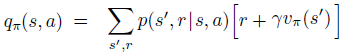
Still we need to figure out a way to quantify the value of each state. This is done by a function called Sate-Value Function:
Details of this equation can be found in this article “Math Behind Reinforcement Learning, the Easy Way”. However what is important to learn about this equation is that the value of each state is the average of discounted future rewards. If we look closely at the equation we see that v(s) is expressed in terms of immediate rewards r and the value of neighboring states v(s’).
The way to understand this equation is as follows:
- when at a state s, consider all possible actions, then,
- for each action a get the probability p(s’, r | s, a) of getting immediate reward r, and moving to neighboring state s’, knowing that we are at state s and we performed action a.
- add the reward r to the discounted value of neighbor state s’ given by γ*v(s’). Multiply the result with p(s’, r | s, a), and we get p(s’, r | s, a)*[r+γ*v(s’)].
- Repeat steps 2 and 3 for all states s’ neighboring s, as well as all the possible rewards r, and compute the sum of the results. Now we have Sum( p(s’, r | s, a)*[r+γ*v(s’)]) over all s’ and r.
- This will give the average of discounted future rewards when taking only one action a. However there are multiple actions to be taken so we have to average over all actions. To do so we multiply by probability 𝜋(a|s) that action a be performed at state s, and we sum over all possible actions in that state.
It sounds complex but this is not the case, it suffices to think that when we are at a state we have a probability to take some action that might lead us to different states with different rewards. So the value of our state is the average of all discounted rewards that we might get when performing all of the possible actions at the current state.
Now we have a function that gives us the value of each state. It tells us how good is to be at each one of them. Of course we still have to make the computation in order to get a number that represents the value of that state.
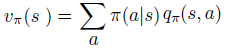
v(s) tells how good to be in state s, but it does not tell how good to perform action a while in state s. This is the purpose of the Action-Value function:
The explication is simple, we take v(s) and instead of performing all actions, we decide to perform only one action. We no more ask ourselves what is the probability of using action a over all possible actions, but we say we will use action a. So the sum of 𝜋(a|s) does not apply anymore. With this logic we reduce v(s) from averaging over all possible actions to simply using one selected action, we denote this as q(s,a).
Notice that q(s,a) checks the value of the action at state s while the values v(s’) of neighboring states are kept unchanged. So in this sense it checks how good this action is in the current state while keeping everything else the same.
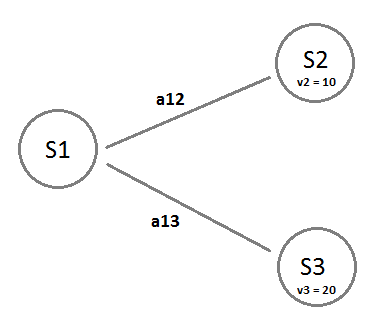
It is also easy to notice that v(s) is the weighted average of q(s,a) over all possible actions at state s.
Policy
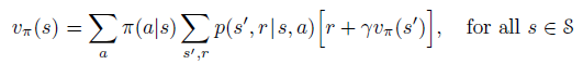
Consider the following case:
a12 is the probability to take the action that leads to S2 from S1. a13 is the probability to take the action that leads to S3 from S1. The value function at S1 and S3 are v2 = 10, v3 = 20 respectiely. We also assume that the reward r = 1 and the discount factor γ = 0.9. Also as simplification, we consider that the transition probabilities is 1, which means when we perform an action we are 100% sure that we will land in the intended state. Under these criteria we can write the value function at S1 which we denote v1 as: v1 = a12*(r + γ *v2) + a13*(r + γ*v3) v1 = a12*(1 + 0.9*10) + a13(1 + 0.9*20) v1 = a12*10 + a13 * 19
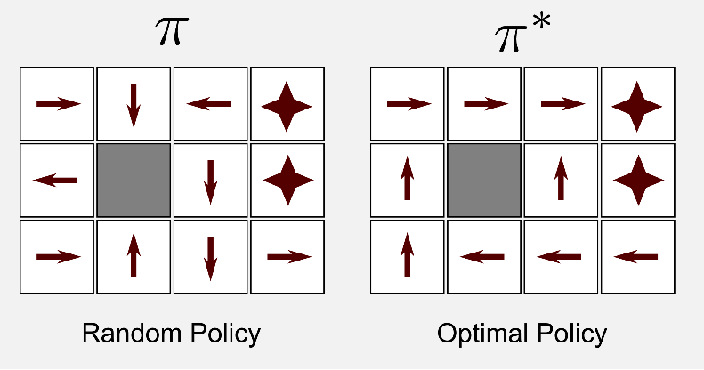
Suppose the action probabilities are a12 = 0.9 and a13 = 0.1 then v1 will be 10.9 . On the other hand if a12 = 0.1 and a13 = 0.9 then v1 will become 18.1! Clearly giving more probability to perform a13 will give better result in terms of the value of the state S1. The act of selecting an action at each state is called “policy” and is denoted as 𝜋.
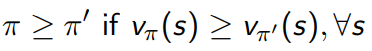
As seen in the example above, some policies are better than others due to the selection of actions over others in one or more states. It is important to note that a policy 𝜋 is better than 𝜋’ if all v(s) under 𝜋 are greater or equal to all v(s) under 𝜋’.
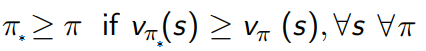
It follows that in order to maximize the collected rewards we have to find the best possible policy, called optimal policy and denoted 𝜋*.
Optimal Value Functions and Policy
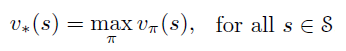
An optimal value state function v*(s) is a function that gives the maximum value at each state among all policies:
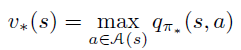
Similarly an optimal action state function q*(s) is the function that gives the maximum q value at each state among all policies:

it follows that
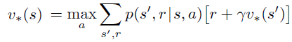
Notice that v(s) is the average of values produced by all actions, while v*(s) is the maximum value that one action can produce among all other actions.
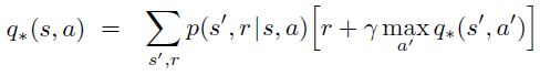
Since q(s,a) is the value produced by a specific action a at state s, q*(s,a) is the value produced by a specific action a at state s, while selecting maximum q values in the other states.
Earlier we said that a policy 𝜋 is better than another policy 𝜋’ if it produces higher or equal v(s) value at each state:
It follows that the optimal policy 𝜋* produces, at each state, higher or equal v(s) values than any other policy 𝜋 .
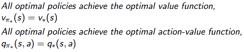
This means that any v(s) and q(s,a) following the optimal policy 𝜋* are equal to v*(s) and q*(s,a) respectively.
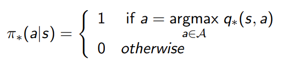
So the question that remains is, how to find the optimal policy 𝜋* ? The optimal policy should always return the action that produces q*(s,a)
- There is always a deterministic optimal policy for any MDP
- If we know q*(s,a) it will be very easy to find 𝜋*.
Note that the optimal policy is not unique, and this can be easily verified. Suppose an agent in the Labyrinth has arrived to a state with 3 possible moves (or actions), go left, go right, or go forward. Suppose going forward leads the agent to a dead end, while going left or right will lead the agent to the exit using the same number of steps. It is clear that there are two optimal policies (not only one) at this state, one that instructs the agent to go left and the other instructs it to go right.
Find the Optimal Policy
Remember that our goal is to find the optimal policy in order for the agent to act accordingly and achieve the maximum rewards. Also recall that knowing v*(s) or q*(s,a) will lead to 𝜋*.
Consider an environment of only 3 interconnected states (S1, S2, S3) with transition probabilities pij to move from Si to Sj, and fixed reward r and discount factor γ.
The value function v(s) is a system of linear equations such as:
v1 = p12*(r + γ *v2) + p13*(r + γ*v3) v2 = p21*(r + γ *v1) + p23*(r + γ*v3) v3 = p31*(r + γ *v1) + p32*(r + γ*v2)
It is easy to solve it using linear algebra. However, when the number of states grows large, it becomes time consuming to solve the system of equation efficiently; actually the complexity becomes O(n³) ! Add to that, we are solving for v*(s) that, unlike v(s), is not linear.
On the other hand there are others ways to solve v(s) using iterative methods:
- Dynamic programming
- Monte-Carlo evaluation
- Temporal-Difference learning
Conclusion
It is easy to be drown into details. What is important to always keep in mind is that the goal is to let the agent collect the maximum reward. To do that we should find the v*(s) or q*(s,a) in order to find the optimal policy 𝜋* (the best way the agent should act). However finding these functions can’t be easily done in Linear Algebra, for this reason we use iterative methods.