Summary

The web content explains the importance and methodology of creating baseline models before training final, more complex time series models to ensure data quality, model performance benchmarks, and the necessity of model complexity.

Abstract

The article emphasizes the critical step of establishing a baseline model in time series forecasting before proceeding with the development of a more sophisticated model. It outlines that a baseline model serves as a benchmark for performance expectations, data quality checks, and the evaluation of the complexity required in the final model. The author suggests that simple statistical models, such as a moving average or a naive forecast, can be used as baseline models for time series data. These models are easy to implement and interpret, providing insights into the data's inherent patterns and potential issues. The article also provides practical Python code snippets to demonstrate how to implement these baseline models, visualize their performance, and calculate evaluation metrics such as Mean Squared Error (MSE) and Root Mean Squared Error (RMSE). The author concludes by cautioning that while these baseline models are valuable for initial benchmarking, they are not suitable for long-term forecasting due to their nature of not truly forecasting into the future.

Opinions

The author believes that baseline models are essential for understanding how a complex model might perform and for identifying potential data quality issues before investing significant time and resources into model development.
It is the author's opinion that if a baseline model outperforms a more complex final model, this could signal problems with the algorithm, features, hyperparameters, or data preprocessing of the final model.
The author suggests that if a baseline model performs on par with a complex model, it may indicate that the added complexity is unnecessary, and a simpler model could suffice.
The author recommends using a naive forecast or a moving average model as baseline models for time series data, emphasizing their ease of use and the ability to reveal the general trend of the data.
The author points out that while baseline models are useful for establishing a performance benchmark, they are not intended for actual long-term forecasting, as they do not account for future variations in the data.

How To: Baseline Models in Time Series

Why (and how) you should create a baseline model before you train your final model

So you’ve collected your data. You’ve outlined the business case, decided on a candidate model (e.g. Random Forest), set up your development environment, and your hands are at the keyboard. You’re ready to build and train your time series model.

Hold up — don’t start just yet. Before you train and test your Random Forest model, you should first train a baseline model.

What is a baseline model?

A baseline model is a simple model used to create a benchmark, or a point of reference, upon which you will be building your final, more complex machine learning model.

Data scientists create baseline models because:

Baseline models can give you a good idea of how a more complex model will perform.
If a baseline model does badly, it could be a sign of an issue with the data quality that needs addressing.
If a baseline model performs better than the final model, it could indicate issues with that algorithm, features, hyperparameters or other data preprocessing.
If the baseline and complex model perform more or less the same, this could indicate that the complex model needs more fine tuning (in features, architecture, or hyperparameters). It could also show that a more complex model isn’t necessary, and a simpler model will suffice.

Typically, a baseline model is a statistical model, such as a moving average model. Alternatively, it is a simpler version of the target model — for example, if you will be training a Random Forest model, you can first train a Decision Tree model as a baseline.

Baseline models in time series

For time series data, there’s a couple of popular options for baseline models that I’d like to share with you. Both of these work well because they assume temporal order of the data and make forecasts according to the data’s patterns.

Naive forecast

The naive forecast is the simplest — it assumes that the next value will be the same as the previous value.

Let’s assume you are building a model trying to predict the weather. I’m going to assume you’ve already loaded in a dataframe df which contains at least the following 2 columns: “Date” and “TemperatureF”. To implement this in Python, begin by separating out your timestamps and target variable, and perform a train/test split.

import numpy as np 

# define the split index
split_time = 1000

# separate the target array and 
# the time/date array
series = np.array(df[‘TemperatureF’])
time = np.array(df[‘Date’])

# train test split
time_train = time[:split_time]
time_test = time[split_time:]

series_train = series[:split_time]
series_test = series[split_time:]

Now that you have your data prepared, you can calculate the naive forecast.

# the naive forecast simply shifts the series by 1 
naive_fcst = series[split_time - 1: -1]

In order to visualize the results and see how the naive forecast performs on the test set, you can use plotly graph objects:

import plotly.graph_objects as go

fig = go.Figure([
        go.Scatter(x=time_test, y=series_test, text='true', name='true'),
        go.Scatter(x=time_test, y=naive_fcst, text='pred', name='pred'),
    ])

fig.show()

Here are my results:

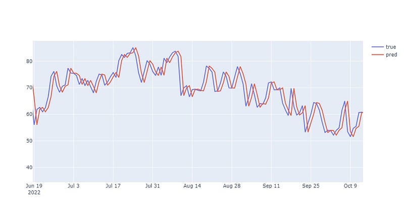
The final step is to calculate metrics which you will use later for benchmarking. Which metrics you choose will depend on your particular problem, but here’s how you can calculate MSE and RMSE:

from sklearn.metrics import mean_squared_error

mse = mean_squared_error(series_test,naive_fcst)
rmse = mean_squared_error(series_test,naive_fcst,squared=False)

print(“MSE:”, mse)
print(“RMSE:”, rmse)

Moving average forecast

A moving average (MA) baseline model predicts that the next data point is the average of the last n data points. Whatever n is is up to you — some common moving averages are the 30-day MA, 60, 90, and 180. This also depends on your use case and domain. In the stock market, some commonly used MAs are 21, 50, 100 and 200. Additionally, if you know you’ll be forecasting 30 days into the future with your final model, you may want to test your baseline using a 30-day MA.

Be sure you research what moving averages are typically used for your specific problem and target outcome.

To implement this in Python, keep the same data structures as before (time and series), and do the following.

First, create the forecast for the entire dataset.

# Initialize a list
forecast = []
window_size = 30

# Compute the moving average based on the window size
for time in range(len(series) - window_size):
    forecast.append(series[time:time + window_size].mean())

# Convert to a numpy array
forecast = np.array(forecast)

Next, separate out the test set from the moving average forecast. You’ll be shifting the forecast array by window_size in order to match it up with the original test set.

moving_avg = forecast[split_time - window_size:]

Do as you did before and plot your results.

fig = go.Figure([
        go.Scatter(x=time_test, y=series_test, text=’true’, name=’true’),
        go.Scatter(x=time_test, y=moving_avg, text=’pred’, name=’pred’),
    ])

fig.show()

It should look something like this, where the moving average is a smoother version of the actual data but which still follows the general trend. This will also vary based on how large your window size is.

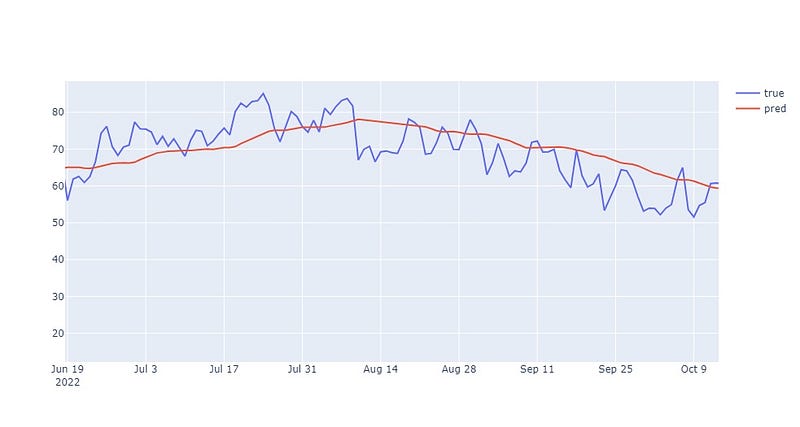
Moving average forecast. Image by author

To get the error metrics, it’s the same process as before except with the moving_avg array.

mse = mean_squared_error(series_test, moving_avg)
rmse = mean_squared_error(series_test,moving_avg,squared=False)

print(“MSE:”, mse)
print(“RMSE:”, rmse)

A word of caution + Conclusion

Although I used the word forecast, notice how I didn’t actually forecast into the future. Since I did a train test split, when predicting on the test set, I already had previous values for each step in the naive prediction. If you were to try and forecast 30 days into the future, a true naive forecast would assume that the next 30 days are the same as the last day or the last data point. This would result in a flat line forecast. The same is true for moving average. Because of this, these techniques aren’t optimal for actually forecasting out long periods of time. However, they are still valuable tools for establishing a baseline and benchmarking what decent performance might look like on a final model.

Baseline models offer a great way to sanity check your code as well as estimate your final model’s ability to reliably predict on a dataset. They can help you detect data errors and aid in the final model selection process. Next time you work with time series data, be sure to run a baseline on it first.