A Complete Guide for Detecting and Dealing with Outliers

6 Methods to Detect the Outliers and 4 different methods to Deal with Them

Outliers can be a big problem in data analysis or machine learning. Only a few outliers can totally alter a machine learning algorithm's performance or totally ruin a visualization. So, it is important to detect outliers and deal with them carefully.

Detecting Outliers

Detecting outliers is not challenging at all. You can detect outliers by using the following:

1. Boxplot
2. Histogram
3. Mean and Standard Deviation
4. IQR (Inter Quartile Range)
5. Z-score
6. Percentile

Before I dive into the detection of outliers, I want to introduce the data I will use for this tutorial today. We will use the ‘tips’ dataset that can be loaded from the seaborn library:

import pandas as pd
import numpy as np
import matplotlib.pyplot as plt
import seaborn as sns

df = sns.load_dataset("tips")
df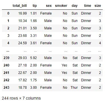

We will primarily focus on the total bill column.

Detection of Outliers

There are quite a few different ways to detect outliers. Some are very simple visualization that only tells you if you have outliers in the data. Some are very specific calculations to tell you the exact data of outliers.

Boxplot

Boxplot shows the outliers by default. Here is the boxplot of the total_bill section:

plt.boxplot(df['total_bill'])
plt.title("Boxplot of Total Bill")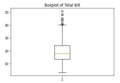

Some of the dots on the upper end are a bit further away. You can consider them outliers. It is not giving you the exact points that are outliers but it shows that there are outliers in this column of data.

Histogram

Looking at the distribution can also tell you if there are outliers in the data:

plt.hist(df['total_bill'])
plt.title("Distribution of Total Bill")
plt.show()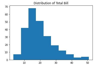

The distribution also shows that the data is skewed and on the right side there are outliers.

From this one, we will perform some specific computations to find out the exact point that is outliers.

Mean and Standard Deviation Method

In this method, we will use mean, standard deviation, and specified factors to find out the outliers.

To start with I will save the total bill column as data:

data = df.total_bill

We will use a factor of three here. Three standard deviations up from the mean and three standard deviations below the mean will be considered outliers. First, get the mean and standard deviation of the data:

mean = np.mean(data)
std = np.std(data)

Now, find the data that are three standard deviations above the mean:

outlier_upper = [i for i in data if i > mean+3*std]
outlier_upper

output:

[48.27, 48.17, 50.81, 48.33]

Here we find out the data that are three standard deviations below the mean:

outlier_lower = [i for i in data if i < mean-3*std]
outlier_lower

Output:

[]

As you can see, we have some outliers on the upper side but on the lower end, there are no outliers in this method.

Here I used 3 std. But if you want you can use a factor of any other number. A factor of 2, 3, or 4 is commonly used. Please feel free to use 2 or 4 and check for the outliers.

Inter Quartile Range

In this method, we need to calculate the first quartile and third quartile to get the interquartile range(IQR). Then we will consider the first quantile minus 1.5 times IQR as the lower limit and the third quartile plus 1.5 times IQR as the upper limit of the data.

data1 = sorted(data)
q1 = np.percentile(data1, 25)
q3 = np.percentile(data1, 75)
IQR = q3-q1
lower = q1-(1.5*IQR)
upper = q3 + (1.5*IQR)

If a value is lower than the lower limit and higher than the upper limit, it will be considered an outlier.

outliers = [i for i in data1 if i > upper or i < lower]

Output:

[40.55, 41.19, 43.11, 44.3, 45.35, 48.17, 48.27, 48.33, 50.81]

These are the outliers in this method.

Z-score

Just fix a z-score threshold and if the z-score is more than that, the data is an outlier.

thres = 2.5
mean = np.mean(data)
std = np.std(data)

outliers = [i for i in data if (i-mean)/std > thres]
outliers

Output:

[48.27, 44.3, 48.17, 50.81, 45.35, 43.11, 48.33]

Percentile Calculation

You can simply fix a percentile for the upper limit and lower limit. In this example, we will consider the lower limit as the tenth percentile and the upper limit as the 90th percentile.

fifth_perc = np.percentile(data, 5)
nintyfifth_perc = np.percentile(data, 95)

outliers = [i for i in data1 if i > nintyfifth_perc or i < fifth_perc]
outliers

Output:

​[3.07,
 5.75,
 7.25,
 7.25,
 7.51,
 7.56,
 7.74,
 8.35,
 8.51,
 8.52,
 8.58,
 8.77,
 9.55,
 38.07,
 38.73,
 39.42,
 40.17,
 40.55,
 41.19,
 43.11,
 44.3,
 45.35,
 48.17,
 48.27,
 48.33,
 50.81]

These are the outliers.

These are all the way to detect outliers I wanted to share today. Let’s see how to deal with outliers now:

Dealing with Outliers

Removing the outliers

This is a common way. Sometimes it is easy to just remove the outliers from the data.

Here I am removing the outliers detected from the last percentile calculation:

no_outliers = [i for i in data if i not in outliers]

Let’s make a boxplot with the no_outliers data:

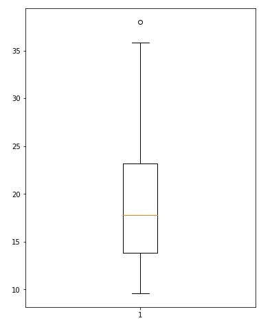
You can see that the outliers are gone.

Percentile Based Flooring and Capping

In the last outlier detection method, the fifth and ninety-fifth percentile was calculated to find the outliers. You can use those percentiles to deal with outliers as well.

The data that is lower than the fifth percentile can be replaced with the fifth percentile and the data that are higher than the ninety-fifth percentile can be replaced with the ninety-fifth percentile value.

data_fixed = np.where(data < tenth_perc, tenth_perc, data)
data_fixed = np.where(data_fixed > nineteeth_perc, nineteeth_perc, data_fixed)

Let’s see the boxplot again with the new data_fixed again

plt.figure(figsize = (6, 8))
plt.boxplot(data_fixed)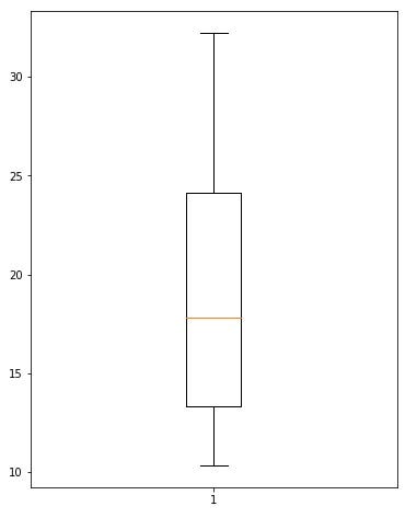

No more outliers.

Binning

Binning the data and categorizing them will totally avoid the outliers. It will make the data categorical instead.

df['total_bill'] = pd.cut(df['total_bill'], bins = [0, 10, 20, 30, 40, 55], labels = ['Very Low', 'Low', 'Average', 'High', 'Very High'])
df['total_bill']

Output:

0          Low
1          Low
2      Average
3      Average
4      Average
        ...   
239    Average
240    Average
241    Average
242        Low
243        Low
Name: total_bill, Length: 244, dtype: category
Categories (5, object): ['Very Low' < 'Low' < 'Average' < 'High' < 'Very High']

The total_bill column is not a continuous variable anymore. It is a categorical variable now.

Considering Null Values

Another way to deal with outliers is to consider them as null values and fill them up using techniques of filling up the null values. Here you will find the tips to deal with null values:

Conclusion

This article wanted to focus on the methods to detect the outliers and the tips to deal with them. I hope this was helpful. If you found any other method more useful, please feel free to share that in the comment section.

More Reading