Scrutinizing Machine Learning Regression Models | Towards AI
Bad and Good Regression Analysis
Regression models are the most popular machine learning models. Regression models are used for predicting target variables on a continuous scale. Regression models find applications in almost every field of study, and as a result, it is one of the most widely used machine learning models. This article will discuss good and bad practices in building a regression model.
We will build a simple linear regression model (no distinction between inliers and outliers which can be handled using more robust regularized regression models such as Lasso regression), then use it to predict house prices using the Housing dataset. We use the output from the model to highlight good and bad practices in regression analysis.
More information about the Housing dataset can be found from the UCI machine learning repository. Jupyter notebook containing all the code can be found on GitHub.
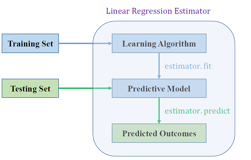
Linear Regression Estimator Using Gradient Descent
In a previous article, we’ve discussed how a simple linear regression model can be built for predicting a continuous outcome variable (y) using a one-dimensional dataset containing a single feature (X): https://readmedium.com/machine-leaning-python-linear-regression-estimator-using-gradient-descent-b0b2c496e463
Implementing a Simple Linear Regression Estimator in Python
class GradientDescent(object):
    """Gradient descent optimizer.
    Parameters
    ------------
    eta : float
        Learning rate (between 0.0 and 1.0)
    n_iter : int
        Passes over the training dataset.

    Attributes
    -----------
    w_ : 1d-array
        Weights after fitting.
    errors_ : list
        Error in every epoch.

    Methods
    -----------
fit(X,y): fit the linear regression model using the data. predict(X): Predict outcome for samples in X. Rsquare(X,y): Returns the R^2 value.
""" def __init__(self, eta=0.01, n_iter=10):
self.eta = eta
self.n_iter = n_iter
def fit(self, X, y):
"""Fit the data.
Parameters
----------
X : {array-like}, shape = [n_points]
Independent variable or predictor.
y : array-like, shape = [n_points]
Outcome of prediction.
Returns
-------
self : object
"""
self.w_ = np.zeros(2)
self.errors_ = []
for i in range(self.n_iter):
errors = 0
for j in range(X.shape[0]):
self.w_[1:] += self.eta*X[j]*(y[j] - self.w_[0] - self.w_[1]*X[j])
self.w_[0] += self.eta*(y[j] - self.w_[0] - self.w_[1]*X[j])
errors += 0.5*(y[j] - self.w_[0] - self.w_[1]*X[j])**2
self.errors_.append(errors)
return self def predict(self, X):
"""Return predicted y values"""
return self.w_[0] + self.w_[1]*X
def Rsquare(self, X,y):
"""Return the Rsquare value"""
y_hat = self.predict(X)
return 1-((y_hat - y)**2).sum()/((y-np.mean(y))**2).sum()Application of Python Estimator: Predicting Housing Prices
a) Import Necessary Libraries
import numpy as np
import matplotlib.pyplot as plt
import pandas as pd
import seaborn as sns
np.set_printoptions(precision=4)
b) Exploring the Housing Dataset
df = pd.read_csv('https://raw.githubusercontent.com/rasbt/'
                 'python-machine-learning-book-2nd-edition'
                 '/master/code/ch10/housing.data.txt',
                 header=None,
sep='\s+')df.columns = ['CRIM', 'ZN', 'INDUS', 'CHAS',
'NOX', 'RM', 'AGE', 'DIS', 'RAD',
'TAX', 'PTRATIO', 'B', 'LSTAT', 'MEDV']
df.head()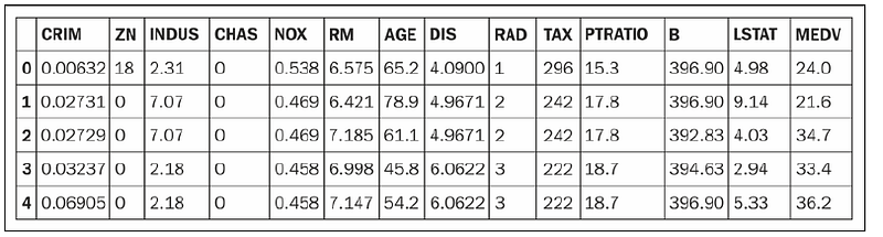
c) Feature Selection and Standardization
cols = ['LSTAT', 'INDUS', 'NOX', 'RM', 'MEDV']
from sklearn.preprocessing import StandardScaler
stdsc = StandardScaler()
X_std = stdsc.fit_transform(df[cols].iloc[:,range(0,5)].values)
# Evaluate the covariance matrixcov_mat =np.cov(X_std.T)
hm = sns.heatmap(cov_mat,
cbar=True,
annot=True,
square=True,
fmt='.2f',
annot_kws={'size': 15},
yticklabels=cols,
xticklabels=cols)plt.tight_layout()
plt.savefig('images/10_04.png', dpi=300)
plt.show()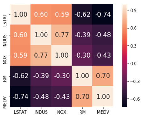
Since we are interested in predicting MEDV (median value of the homes), we see that the strongest correlation is found with RM (average number of rooms per dwelling). So in our model, we shall use RM as the predictor variable, and MEDV as the target variable:
X=X_std[:,3] # we use RM as our predictor variable
y=X_std[:,4] # we use MEDV as our target variable
d) Calculate R-square Values for Different Learning Rates
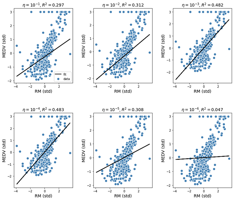
[GradientDescent(eta=k, n_iter=100).fit(X,y).Rsquare(X,y) for k in [0.1,0.01,0.001,0.0001,0.00001,0.000001]]We obtained the following output:
[0.297,0.312,0.482,0.483,0.308,0.047]e) Fit, Predict, and Hyperparameter Tuning
np.set_printoptions(precision=1)
# plot with various axes scales
plt.figure(figsize=(10,8))
# fig 1
plt.subplot(231)
plt.scatter(X,y,c='steelblue', edgecolor='white', s=70,label='data')
plt.plot(X, GradientDescent(eta=0.1, n_iter=100).fit(X,y).predict(X),color='black', lw=2,label='fit')
plt.title('$\eta = 10^{-1}, R^2 = 0.297$ ',size=14)
plt.grid(False)
plt.xlabel('RM (std)',size=14)
plt.ylabel('MEDV (std)',size=14)
plt.legend()# fig 2
plt.subplot(232)
plt.scatter(X,y,c='steelblue', edgecolor='white', s=70)
plt.plot(X, GradientDescent(eta=0.01, n_iter=100).fit(X,y).predict(X),color='black', lw=2)
plt.title('$\eta = 10^{-2},R^2 = 0.312$',size=14)
plt.grid(False)
plt.xlabel('RM (std)',size=14)
plt.ylabel('MEDV (std)',size=14)# fig 3
plt.subplot(233)
plt.scatter(X,y,c='steelblue', edgecolor='white', s=70)
plt.plot(X,GradientDescent(eta=0.001, n_iter=100).fit(X,y).predict(X),color='black', lw=2)
plt.title('$\eta =10^{-3},R^2 = 0.482$',size=14)
plt.grid(False)
plt.xlabel('RM (std)',size=14)
plt.ylabel('MEDV (std)',size=14)# fig 4
plt.subplot(234)
plt.scatter(X,y,c='steelblue', edgecolor='white', s=70)
plt.plot(X, GradientDescent(eta=0.0001, n_iter=100).fit(X,y).predict(X),color='black', lw=2)
plt.title('$\eta = 10^{-4}, R^2 = 0.483$ ',size=14)
plt.grid(False)
plt.xlabel('RM (std)',size=14)
plt.ylabel('MEDV (std)',size=14)# fig 5
plt.subplot(235)
plt.scatter(X,y,c='steelblue', edgecolor='white', s=70)
plt.plot(X, GradientDescent(eta=0.00001, n_iter=100).fit(X,y).predict(X),color='black', lw=2)
plt.title('$\eta = 10^{-5},R^2 = 0.308$',size=14)
plt.grid(False)
plt.xlabel('RM (std)',size=14)
plt.ylabel('MEDV (std)',size=14)# fig 6
plt.subplot(236)
plt.scatter(X,y,c='steelblue', edgecolor='white', s=70)
plt.plot(X,GradientDescent(eta=0.000001, n_iter=100).fit(X,y).predict(X),color='black', lw=2)
plt.title('$\eta =10^{-6},R^2 = 0.047$',size=14)
plt.grid(False)
plt.xlabel('RM (std)',size=14)
plt.ylabel('MEDV (std)',size=14)plt.subplots_adjust(top=0.92, bottom=0.08, left=0.10, right=0.95, hspace=0.4, wspace=0.35)plt.show()Here is the output:
General Remarks and Conclusion
Using our simple regression model, we could see that the reliability of our model depends on hyperparameter tuning. If we just pick a random value for the learning rate such as eta = 0.1, this would lead to a poor model. Choosing a value for eta too small, such as eta = 0.00001 also produces a bad model. Our analysis shows that the best choice is when eta = 0.0001, as can be seen from the R-square values.
What makes the difference between a good and a bad regression analysis depends on one’s ability to understand all the details of the model including knowledge about different hyperparameters and how these parameters can be tuned in order to obtain the model with the best performance. Using any machine learning model as a black box without fully understanding the intricacies of the model will lead to a falsified model.
References:
- “Machine Learning: Python Linear Regression Estimator Using Gradient Descent”, Benjamin O. Tayo (https://readmedium.com/machine-leaning-python-linear-regression-estimator-using-gradient-descent-b0b2c496e463).
2. “Python Machine Learning”, 2nd Edition, Sebastian Raschka.
3. UCI machine learning repository at https://archive.ics.uci.edu/ml/machine-learning-databases/housing/.
4. Jupyter notebook containing the entire code used in this article is found here: https://github.com/bot13956/python-linear-regression-estimator.


