
Backpropagation
From mystery to mastery: Decoding the engine behind Neural Networks.

The term backpropagation, short for “backward propagation of errors,” is a supervised learning algorithm used to minimize errors in predictions made by neural networks.
In principle, Backpropagation is a chain-rule application that can be used to compute gradients of loss functions in relation to model parameters. The mechanism operates in two main phases:
The forward pass and the backward pass.
1.- Forward pass An input is passed through the neural network layers to generate a prediction. The prediction is then compared with the real label to calculate an error.
2.- Backward pass To adjust the weights so that the error is minimized, the backward pass starts with this error and works backward through the network. The neural network then, gradually improves its prediction through iterative adjustments using optimization algorithms such as gradient descent.
Let’s look at a more precise explanation:
Backpropagation is essentially an application of the chain rule of calculus to compute the gradient concerning each weight in the network.
There are two main concepts that you must understand before delving deeper into how backpropagation works, the chain rule and the gradient.
1.- Chain rule
The chain rule is a fundamental concept in calculus that describes how to compute the derivative of composite functions. It’s especially useful when functions are nested within one another.
Basic Idea Suppose you have two functions y = g(u) and u = f(x) that are composed to form y = g(f(x)). The chain rule provides a formula to compute the derivative of y with respect to x by considering the “intermediate” function u.
Mathematical Formulation If y is a function of u and u is a function of x, then the derivative of y with respect x is given by:
This can be extended to two functions (or more). Suppose y is a function of u, u is a function of v, and v is a function of x. Then:
Let’s see an example to understand it better:
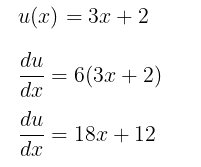
Example Given the functions:
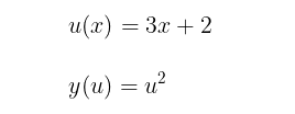
Find the derivative of y with respect to x, denoted dx/dy.
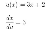
Step 1: Find du/dx
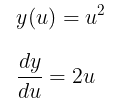
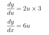
Step 2: Find du/dy
Step 3: Apply the Chain Rule
Step 4: Plugging in what we found
Step 5: Replace u with the original function of x:
Solution:
The derivative of y with respect to x is:
This result describes how a small change in x affects y through its effect on u.
2.- Gradient
Derivative In the context of a single-variable function, you might recall the concept of a derivative, which gives the slope of the tangent line at a point.
Gradient When dealing with functions of multiple variables, the gradient is used, which is a generalization of the derivative. It gives the direction of the steepest ascent, and its magnitude represents the rate of increase in that path.
Mathematical formulation The gradient can be represented with a function f(x) where x = (x1, x2, …, xn) is a vector in R. The gradient of f, often denoted by ∇f, is defined as:
Example Consider the following function:
We want to find the gradient of f at a particular point, say (1,2).
Step 1: Compute the Partial Derivatives
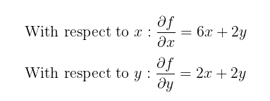
Step 2: Evaluate the Partial Derivatives at the Point (1,2)
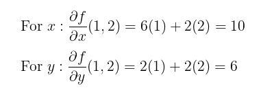
Step 3: Construct the Gradient
Using the results from Step 2, the gradient of f at the point (1,2) is: ∇f(1,2) = (10,6)
Interpretation
At point (1,2), for every unit increase in the x direction, the function will increase by 10 units. Similarly, for every unit increase in the y direction, the function will increase by 6 units.
- Magnitude
The magnitude (or length) of the gradient vector indicates the steepness of the ascent. A larger magnitude implies a steeper ascent. The magnitude can be computed using the Pythagorean theorem. For the vector (10,6) it can be calculated in the following way:
This means that when you move from the point (1,2) in the direction of the gradient vector (10,6), for each tiny unit step you take, the function value f(x,y) will increase approximately by 11.66 units.
Chain rule and gradient in backpropagation
Think of neural networks as giant composite functions, composed of a very big number of interconnected neurons.
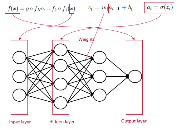
Chain rule and gradient Each layer builds upon the information from its predecessor, finishing in the output layer. To dissect and understand these layers, we employ the chain rule.
Through this decomposition, we can explain the impact of each weight on the overall loss function by computing the gradient.
For example, if we want to know how a change in a weight from the first layer impacts the final loss, we have to consider:
How this changes the first layer’s output → then how this change affects the second layer’s output → how this affects the third layer’s output → and so on until the final layer.
This is a typical scenario where you apply the chain rule and then compute the gradient, this will tell us how much the overall loss will change with a small variation in that specific weight.
Backpropagation (the whole process)
Step 1: Compute the Forward Pass Begin by passing an input through the network to get its output. This gives the activations at every layer.
Step 2: Compute the Loss Calculate the difference between the predicted output and the actual target value, using a loss function.
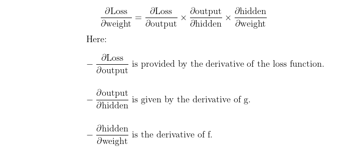
Step 3: Backward Pass For each weight, we want to compute how much the loss changes if the weight is changed. This can be expressed as:

If you expand this gradient using the chain rule, you’ll see that it’s a product of gradients from the output layer back to the layer containing the weight.
For instance, suppose our network has the form:

To compute the gradient of the loss with respect to a weight in the function f, we’d use the chain rule as:
Step 4: Adjust the weights
With these gradients in hand, we adjust the weights in the direction that reduces the loss. This is typically done using an optimization algorithm like Gradient Descent or one of its variants (like Adam or RMSprop).
The above process is carried out for every weight in the network.
Now let’s see an example using calculus and Python to have an idea about how this algorithm is computed:
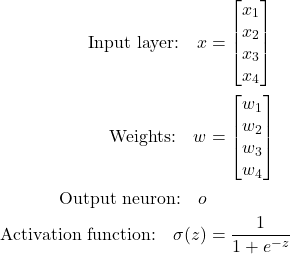
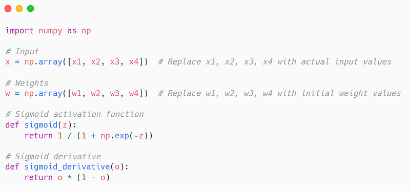
Example of backpropagation I will illustrate backpropagation with a simple feedforward neural network consisting of an input layer with 4 neurons, and one output layer (i.e., no hidden layers). For simplicity, we’ll also assume there’s just a single neuron in the output layer.
Parameters of our neural network:
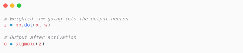
Step 1: Forward propagation
Given an input vector x, the weighted sum going into the output neuron is:

Then, the output of the neuron after the activation function is:
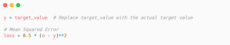
Step 2: Loss Function
Let’s assume we’re using Mean Squared Error (MSE) as our loss function:
Step 3: Backpropagation:
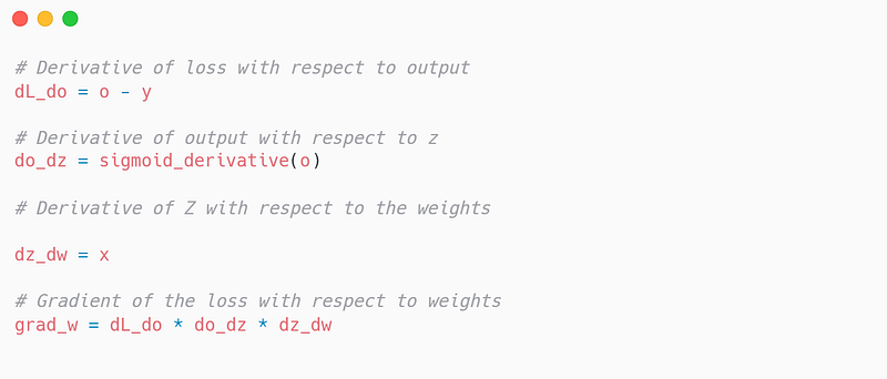
Now, to adjust the weights, we need to compute the derivative of the loss with respect to each weight.
Using the chain rule:
Where:
Multiplying these terms together, we get the gradient for weight wi:
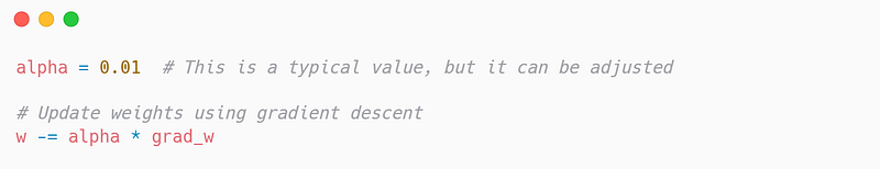
Step 4: Weight Update
Finally, to update the weight wi, we’ll use gradient descent where α is the learning rate:
This process will be repeated with weights w1, w2, w3, and w4.
Bibliography:
- Kostadinov, S. (2019, Aug 8). Understanding Backpropagation Algorithm. Towards Data Science.
- Wikipedia contributors. (2022, 28 November). Backpropagation. In Wikipedia.
- 3Blue1Brown. (2017, Nov 3). But what is backpropagation really doing? | Deep learning, chapter 3. YouTube.
- Andrej Karpathy. (2016, Jan 14). CS231n Winter 2016: Lecture 4: Backpropagation, Neural Networks 1. YouTube.
Thanks for reading! If you like the article make sure to clap (up to 50!) and follow me on Medium to stay updated with my new publications.


