Back-propagation Demystified in 7 Minutes
In the past 10 years, the best-performing machine learning implementations such as the facial recognition and the speech recognizers have resulted from a technique called “deep learning.” Deep learning is composed of neural networks, which are a means to perform some task by analyzing training examples. How do neurons of the neural networks learn from training examples?
There are three steps.
- Let your neural network guess the output.
- Evaluate how well your network did.
- Modify/Teach your neural network based on the evaluation from step 2. a.k.a. backpropagation
Step 1. Let your NN guess by forward pass.
When you make prediction using neural networks,
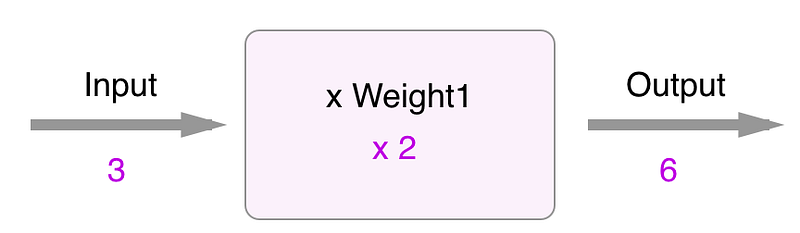
In order to train a neural network, you need to evaluate how good your prediction was. That’s when a loss function comes in to play.
Step 2. Evaluate how well your network did.
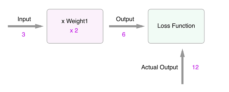
Loss functions compare what the output is supposed to be with the prediction that was made from the neural network. One of the most common examples of loss functions would be a mean squared error (MSE). It calculates the difference between the truth and prediction and square it. The reason that you square the result is to make the negative difference not relevant.

If you have multiple predictions and truths, this is what you do.
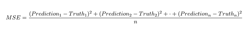
In this case,

your loss function would give you the error of 36. You want to make your mean squared error as low as possible. Ideally, you want to make it 0, but we’d be satisfied with any value that is close enough to it.
Step 3. Modify/Teach your neural network
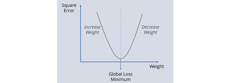
Your error value is somewhere on the graph below. You might have to either increase weight or decrease weight for you to reach the minimum error possible. This step is called back-propagation. In order to achieve this goal of reaching the minimum error, there are multiple ways you can take. I will discuss two popular approaches.
Approach 1. Take a derivative and set it equal to 0 and solve for it
In calculus class, we learned that in order to reach the optimal point, you can take a derivative of the function with respect to the input, set it equal to 0 and solve for it.

By solving for w, we get w = truth/input. In this case, the truth was 12, the input was 3, so our w becomes 4. We finally taught our neural network!
This approach is simple and fast but it doesn’t always work because most loss functions don’t have closed form derivatives.
Approach 2. Gradient Descent
Gradient in calculus is a collective of partial derivatives. And it’s proven that gradient is the direction of the steepest ascent. If those previous sentences were confusing to you, all you need to know is when you take a derivative, that value is telling you what direction to take to get to the highest point on your graph. However, we want to get to the lowest point, because our graph’s y-axis is error and we want to minimize the error, we will go to the opposite direction of the gradient by taking a negative value of the gradient.
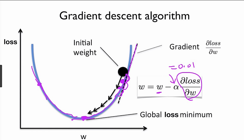
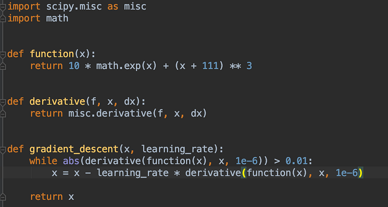
You start somewhere on the graph, and you keep going the opposite direction of the gradient in order to reach the minimum. You can see the gradient descent in python implementation below.
Chain Rule
In the example above, there was only one weight, which is not common in the real world. Let’s go over an example with multiple weights and how chain rule is applied to calculate the derivatives.
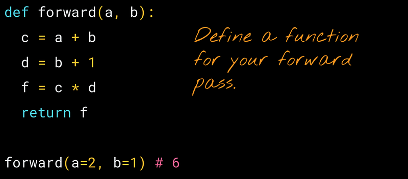
We will represent weights and loss function as a graph. Please note that “a” and “b” represent weights and “f” represents a loss function we want to minimize. We will see how adjusting the weights affects the output using the chain rule.
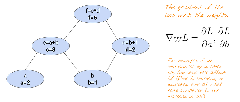
The gradient of the loss with respect to the weights can be represented in two ways, because there are two weights. If you were to define a function for the above forward pass, it’d be like this:
Let’s start with calculating dL/da = df/da. The problem is the loss function f does not know about a. Every node is only aware of its adjacent nodes.
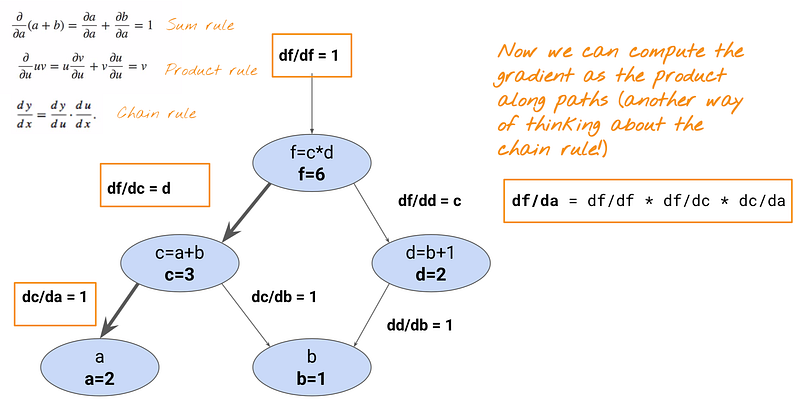
Therefore, in order to calculate df/da, you need to use the chain rule. Simply put, the chain rule is used when you have composite functions.
Since df/da cannot be calculated directly from the f node, which does not know about the node a, you’ll do df/da = df/dc * dc/da.
Now, let us calculate dL/db = df/db. Since there are two edges coming out of the node b, when we back-propagate, we need to use the sum rule to add two paths to the node b.
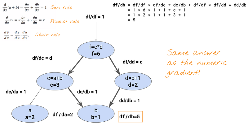
Each path can be calculated by using the chain rule: df/dc * dc/db and df/dd * dd/db and we can sum them at the end.
In reality, those weights are vectorized, so all weights are calculated at the same time when we do back-propagation.
Complexity of Back Propagation
Let’s think about our neural network as a graph. A node represents an operation and an edge represents a weight. In order to calculate gradient for every weight, every edge has to be visited at least once. Therefore, the complexity of back propagation is linear in the number of edges.
How to reach the minimum fast?
Sometimes it may take awhile to reach the minimum while backpropagating. There are some tricks/adjustments you can make to reach the minimum fast.
- Adjust the learning Rates
Learning rates are the value you multiply by the gradient to be subtracted from the loss function in order to reach the minimum.
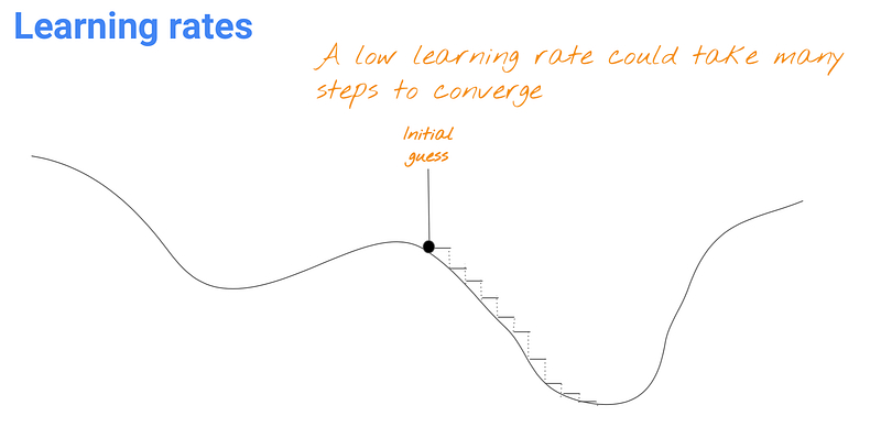
If you make the learning rate small, you can ensure to reach the minimum, but it’d take awhile.
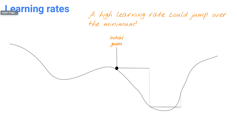
If your learning rate is too big, you might not be able to reach the minimum, because you can jump over the minimum. So you want to make the learning rate big enough to converge to get close enough to the minimum quickly and adjust it later to be small enough to reach the minimum.
2. Adjust the momentum
With the use of momentum, the gradient of the past steps are accumulated instead of using only the gradient of the current step to guide the search.
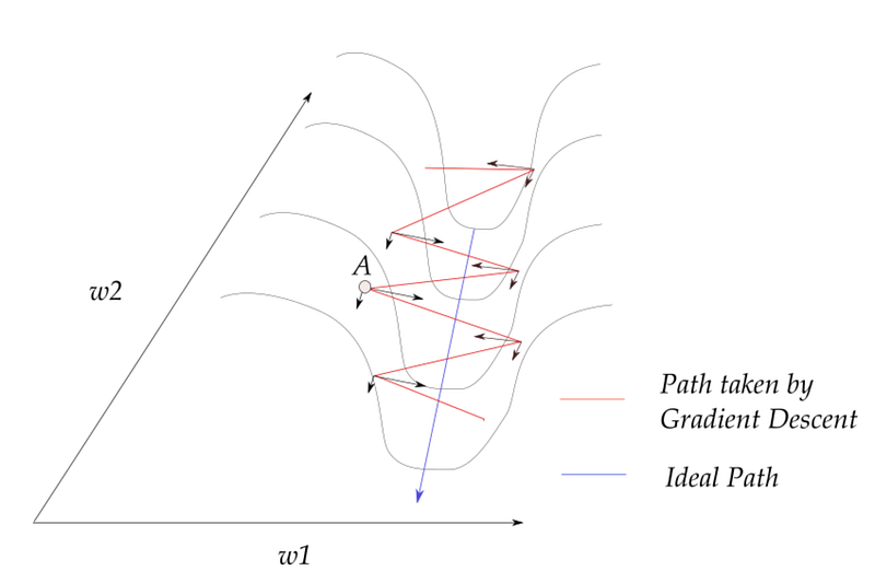
The momentum is used for the following reason. In the diagram above, consider the point A. If we were to sum those vectors up, the opposite directions cancel out, so the components along the w1 direction cancels out, but the w2 direction increases, which is the ideal path we want to make towards the optimum.
3. Change the batch size
Batch is the entire training set to compute gradient. Instead of using the entire batch, you can either choose random training samples at a time (stochastic) or use a small batch of data at a time (mini-batch).
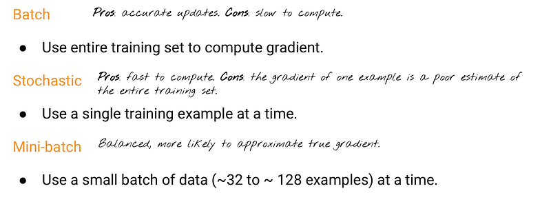
Stochastic method significantly decreases the time of computing gradient descent; however, it’s using only one example at a time, so its path to an optimum is noisier and can be more random than that of the batch gradient. But it doesn’t have a huge impact as we don’t care what kind of path this method is taking (only for now) as long as the minimum point has been reached with a shorter training time.
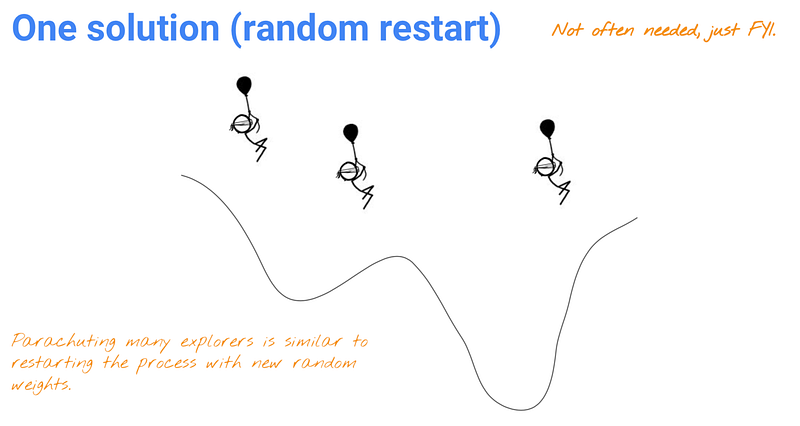
Local and Global Minimum
If we have multiple minima, we want to reach the global minimum. However, it is possible that we can get trapped in a local minimum like the diagram below.
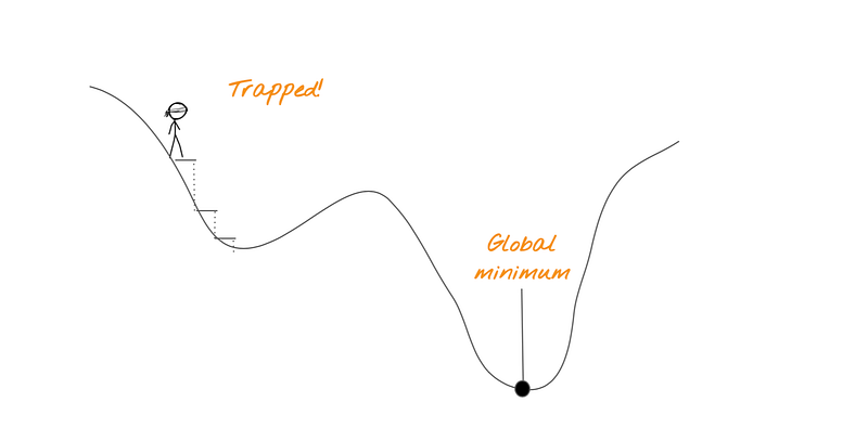
In that case, the best way for you to get out of the local minimum is restart randomly. A hack to get out of a local minimum is to do random restart, which raises the probability of reaching a minimum somewhere else.