Automating Time Series Forecasting

Using PMDArima for Time Series Forecasting

Time-series forecasting is one of the important applications for Machine Learning and Deep Learning. There are multiple models which can be used for time series forecasting like Arima, Prophet, Holt-Winters, etc. Multiple Python libraries can be used for loading these models and using them but they are not user-friendly and are difficult to use.

PMDArima is an open-source Python library that is used for time series forecasting and also helps in creating time series plots. It is easy to use and generates time-series forecast on the ARIMA model.

In this article, we will explore PMDArima and generate a time-series forecast using it.

Let’s get started…

Installing required libraries

We will start by installing a PMDArima library by using pip. For downloading the data we will use the yfinance library. The command given below will do that.

!pip install pmdarima
!pip install yfinance

Importing required libraries

In this step, we will import the required libraries for loading a dataset and creating the ARIMA model.

import yfinance as yfimport numpy as np
import pandas as pd
import matplotlib.pyplot as plt
%matplotlib inline
import pmdarima as pm
from pmdarima.arima import ndiffs
from sklearn.metrics import mean_squared_error
from pmdarima.metrics import smape

Downloading dataset

For downloading the dataset we will use Yahoo finance. You can follow the code given below for downloading the data for the particular ticker and can also follow the article to understand yfinance and its functionalities.

hindpetro = yf.Ticker("HINDPETRO.NS")
df = hindpetro.history(period="max")
df = df.reset_index()
df.head()

Data Preprocessing & Modelling

Next, we will preprocess the data by splitting it into test and train. Also, we will define the function for forecasting.

train_len = int(df.shape[0] * 0.8)
train_data, test_data = df[:train_len], df[train_len:]
y_train = train_data['Open'].values
y_test = test_data['Open'].values
kpss_diffs = ndiffs(y_train, alpha=0.05, test='kpss', max_d=6)
adf_diffs = ndiffs(y_train, alpha=0.05, test='adf', max_d=6)
n_diffs = max(adf_diffs, kpss_diffs)

model = auto

def forecast_one_step():
  fc, conf_int = model.predict(n_periods=1, return_conf_int=True)
  return (fc.tolist()[0],np.asarray(conf_int).tolist()[0])

forecasts = []
confidence_intervals = []
for new_ob in y_test:
  fc, conf = forecast_one_step()
  forecasts.append(fc)
  confidence_intervals.append(conf)
  model.update(new_ob)

Visualizing Actual Vs Predicted Values

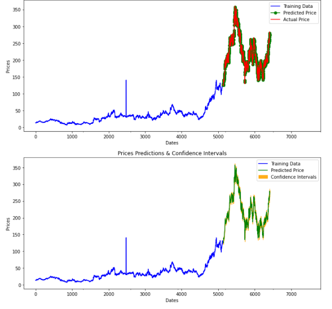
In this step, we will visualize the actual vs. predicted values given by the model. Similarly, we will also plot the confidence intervals with the predicted values.

fig, axes = plt.subplots(2, 1, figsize=(12, 12))

# --------------------- Actual vs. Predicted --------------------------
axes[0].plot(y_train, color='blue', label='Training Data')
axes[0].plot(test_data.index, forecasts, color='green', marker='o', label='Predicted Price')
axes[0].plot(test_data.index, y_test, color='red', label='Actual Price')
axes[0].set_title('Prediction')
axes[0].set_xlabel('Dates')
axes[0].set_ylabel('Prices')
axes[0].set_xticks(np.arange(0, 7982, 1300).tolist(), df['Date'][0:7982:1300].tolist())
axes[0].legend()

# ------------------ Predicted with confidence intervals ----------------
axes[1].plot(y_train, color='blue', label='Training Data')
axes[1].plot(test_data.index, forecasts, color='green', label='Predicted Price')
axes[1].set_title('Prices Predictions & Confidence Intervals')
axes[1].set_xlabel('Dates')
axes[1].set_ylabel('Prices')
conf_int = np.asarray(confidence_intervals)
axes[1].fill_between(test_data.index,conf_int[:, 0], conf_int[:, 1],alpha=0.9, color='orange',label="Confidence Intervals")
axes[1].set_xticks(np.arange(0, 7982, 1300).tolist(), df['Date'][0:7982:1300].tolist())
axes[1].legend()

Here we can clearly visualize the predicted and actual values and use them for analysis. Go ahead try this with different datasets and perform forecasting and visualizations using PMDArima. In case you find any difficulty please let me know in the response section.

This article is in collaboration with Piyush Ingale.

Before You Go

Thanks for reading! If you want to get in touch with me, feel free to reach me at [email protected] or my LinkedIn Profile. You can view my Github profile for different data science projects and packages tutorials. Also, feel free to explore my profile and read different articles I have written related to Data Science.