Automating GIS and remote sensing workflows with open python libraries

A hands-on guide for implementing some of the most beloved tools in the spatial python community

Over my career I’ve worked on many geospatial related projects using the ArcGIS platform, which I absolutely love. That means I get to consult in projects with cutting-edge geospatial technologies, like Multidimensional Rasters, Deep Learning, and spatial IoT automation. With that in mind, I always try to keep track of how to perform the same operations I’m working on without Esri’s beautifully crafted systems.

Over the last few weekends during an exceptionally tedious quarantine I've worked on this little script that would reproduce something I've been developing with ESRI's Living Atlas to achieve NDVI Zonal Statistics (Normalized Difference Vegetation Index, a classic in Remote Sensing) for rural land plots.

The plan here was to perform an entire geoprocessing and remote sensing routine without having to resort to any GIS Desktop software. We're starting out with a layer that contains some parcels in which we're intersted and a layer with protected areas where special legislation applies. Nothing else is allowed outside python! This is our plan du jour:

1. Check the parcels geojson layer for invalid geometries and correcting those;
2. Calculate the area for each parcel in hectares;
3. Verify for each parcel if it intersects any protected areas;
4. Calculate the area of intersection for each parcel and insert the name of the protected area on the parcel's attributes;
5. Get the latest five Sentinel-2 satellite imagery with no clouds;
6. Calculate the NDVI on each image;
7. Calculate zonal statistics (mean, min, max and std. dev.) for the NDVI on each parcel;
8. Create a map showing the results clipped in each parcel.

Let's get started

So. First things first. We have to import the geojson file that has the land plots stored in it. For that, we'll be using the geopandas library. If you're not familiar with it, my advice is get acquainted with it. Geopandas basically emulates the functions we've been using in classic GIS Desktop softwares (GRASS, GDAL, ArcGIS, QGIS…) in python in a way consistent with pandas — a very popular tool among data scientists — to allow spatial operations on geometric types.

In order to import our geojson, the first thing we must note are the data types in geopandas. Basically, when we ran the .read_file method, we assigned a geodataframe type to the polygons variable. Inside every geodataframe there will always be a geoseries , which we can access via the .geometry method. Once we find the geoseries , we can make use of the .isvalid method, that produces a list of True/False values for each record in our series.

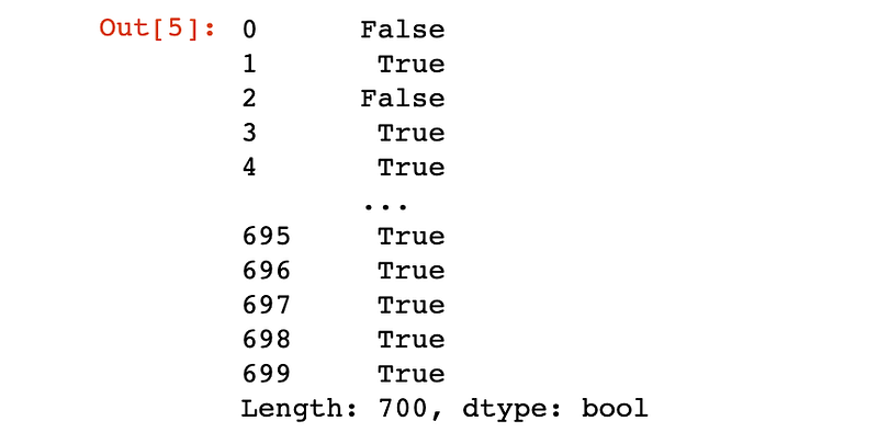
And of course there are invalid geometries hanging in our dataset. It comes as no surprise, since those land plots came from the CAR Registry, where every rural land owner in Brazil have to self-declare the extent of their own properties.

So, how do we fix that? Maybe you're used to running the excelent invalid geometries checking tools present in ArcGIS or QGIS, which generate even a report on what the problem was with each record in a table. But we don't have access to those in geopandas. Instead, we'll do a little trick to correct the geometries, by applying a 0 meter buffer to all geometries.

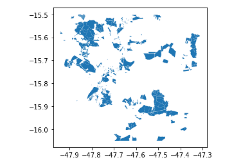
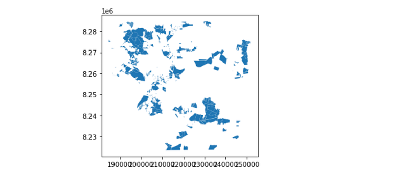
And now we’ll finally get to take a look at our polygons, by using the .plot method, which is actually inherited from thematplotlib components in geopandas .

This is a fast and useful way to get a quick notion of what our data looks like spatially, but it's not the same as a map.

Calculating areas

Since we want to know the area of each of our land plots in hectares, we need to make sure our geodataframe is in a Projected Coordinate System. If you're not familiar with coordinate reference systems (CRS), the bare minimum you need to know is that Geographic Coordinate Systems operate in degrees (like latitude and longitude) and Projected Coordinate Systems operate in distances, enabling us to calculate areas using the metric system. From the plotted graph we just created we can see that the polygons are probably plotted accordingly to latitude and longitude, somewhere around -15.7°, -47.7°. If we run print(polygons.crs) we'll get epsg:4326 as response. There are many coordinate systems available, so the EPSG system is a very good way to keep track of them; 4326 means our geodataframe is in the WGS84 Coordinate System — a Geographic Coordinate System indeed.

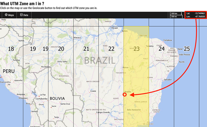
So we do need to transform the coordinate system of our geodataframe. To do that, we must first decide which system we'll transform it into. At this point I'm very used to converting from one system to another, but if you're a bit lost, a good way to choose a projected coordinate system is just using the Universal Transverse of Mercator Projection of the WGS84 system. So all you have to do is find out in which UTM Zone your data is in, so you know that's the zone where your data will have the least area distortion. A good way to do that is this little web application.

So all that's left is visiting the EPSG Authority website and checking the EPSG code for our chosen projection. Next, we need to define a new geodataframe variable using the .to_crs method.

We can now finally create a new column in that new geodataframe, which I named area_ha and calculate the area (in meters, since we're using a UTM projection) that we'll have to divide by 10,000 for it to be in hectares.

Checking for overlays

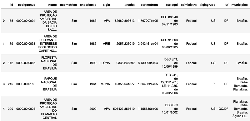
We can now import the second layer we were provided with, the one with all the protected areas (UCs, or Unidades de Conservação) that might represent legal restrictions to agricultural use in the land plots we're analysing. We'll import it just like we did with the previous geojson. The main difference this time is that this piece of data actually has a lot more fields, with the name of the protected area as well as the date of creation and more legal stuff.

We're interested in getting all that rich information into the attribute table of the land plots intersecting a given protected area. Geopandas actually makes that very easy to do, with the overlay method. It does literally exactly what we're looking for. In our case, it will create a new geodataframe with one record for each intersecting part of each land plot, with the information about the protected area it intersected. With that we can calculate a new field for the area of intersection in hectares, just like we did before.

Now for the remote sensing bit

We're done dealing with the GIS bit of this article, and now things get interesting. We want to get a good sense of how the vegetation is doing in each land plot, so we'll try to get the latest (free) satellite imagery we can get and run some analyses with it. There are many options of free satellite imagery, like the Landsat family, but ESA's Sentinel2 mission provides free imagery in a decent spatial scale (20x20m pixel).

To access that, there's more than one library we could use. The Sentinel Hub is a solid one, ArcGIS Living Atlas is another one. But my personal choice is Google Earth Engine for two simple reasons: with small changes we can access data from Landsat and Sentinel with the same code, plus it's (still) free to use — but let us not forget what happened with Google Maps API. The real downside here is that the GEE's python API is poorly documented.

What we want to do is fairly simple. We have to call the Sentinel 2 Image Collection from GEE, filter it for area of interest, date and cloud percentage, and get the latest five in the collection. In order to get the area of interest, we have to run one more command with geopandas, the .total_bounds method, which will give us the coordinates for a rectangle that contains the full extent of our land plots.

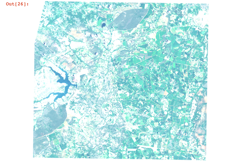
We have taken those five latest images and stored them in our collectionList variable. But let's have a look to make sure the satellite imagery actually corresponds to our expectations. To do that, let's use Earth Engine's .Image , set it to a RGB composition — in Sentinel 2, that means using the bands 4, 3 and 2 — and plot it using Ipython's .display .

Calculating the NDVI

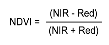
This bit is actually pretty simple. GEE makes it very easy to calculate normalized differences, which is precisely what NDVI is:

The normalized difference vegetation index (NDVI) is a simple graphical indicator that assesses whether or not the target being observed contains live green vegetation. Healthy vegetation (chlorophyll) reflects more near-infrared (NIR) and green light compared to other wavelengths. But it absorbs more red and blue light.

NDVI quantifies vegetation by measuring the difference between near-infrared (which vegetation strongly reflects) and red light (which vegetation absorbs). Satellite sensors like Landsat and Sentinel-2 both have the necessary bands with NIR and red.

In GEE, we just need to use the .normalizedDifference method with the right bands. In our case, it's the bands 8 (NIR) and 4 (Red). Normally, that would be it, but I'm an old-fashioned GIS geek, so I need to have a look at my data in a map to make sure it went ok.

For that, I'll create a simple Folium map — a way to render Leaflet maps with python — and load both the NDVI raster and the land plots geojson to it.

Zonal Statistics is fun

We're almost through. What we need to do now is resume the NDVI data we just calculated for the five Sentinel 2 images in each land plot. Folks in the remote sensing have been doing this for many years, with something called Zonal Statistics. This tool is present in many GIS Desktop softwares, and it's possible even in GEE python API — again, poorly documented. For simplicity, ease of access and liability, my preferred tool for this is actually rasterstats.

The problem is, so far we've been dealing with GEE own format for dealing with imagery. And rasterstats will be needing those oldschool .TIF files. So we gotta export our imagery to a local folder.

Finally, this is where the magic happens. Let us have a little for loop that opens each local NDVI raster file, calculates the stats for each land plot, and then append the results for mean, minimum, maximum and standard deviation to a pandas' dataframe.

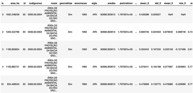
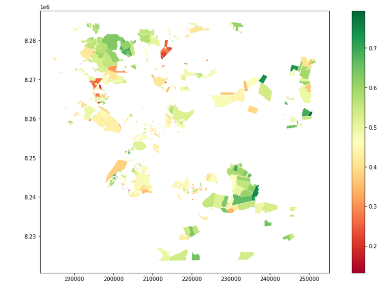
We can now visualize the NDVI statistics in each of our land plots by plotting our data, just like before, except this time we can tell matplotlib which column and which color scheme to use. Since the results seem ok, we can export the geodataframe to a geojson file and share with our not-so-tech colleagues.

That's all folks

That's it for this piece! We have successfully implemented classic geoprocessing and remote sensing workflows without having to use ArcGIS or QGIS once! You can find this whole workflow in my Github page. If you have questions or suggestions, don't hesitate to drop me a line anytime!

If you enjoyed this article, consider buying me a coffee so I keep writing more of those!