
Autoencoders vs t-SNE for Dimensionality Reduction
While preserving spatial relationships between data points in both lower and higher dimensions

Autoencoders (AEs) and t-SNE are two main techniques for dimensionality reduction.
Autoencoders are a type of neural network architecture with many practical applications. Dimensionality reduction is one of them. Autoencoders can be used for dimensionality reduction in non-linear data.
t-SNE is also a non-linear dimensionality reduction technique that can be used for visualizing high-dimensional data in a lower-dimensional space to find important clusters or groups in the data.
Both t-SNE and autoencoders can handle non-linear data which is very common in real-world applications.
However, autoencoders need a very large amount of data and computational resources to train the algorithm as it is a neural network architecture. In contrast, t-SNE is a general machine-learning algorithm that only needs a very small amount of data to train the algorithm.
In particular, t-SNE can preserve the spatial relationship between data points in both higher and lower dimensions after reducing the dimensionality of the data. It means that the nearby data points of the same class in the original dimension will still be nearby in the lower dimension. Therefore, t-SNE is mostly used for visualizing clusters in the data.
The same “spatial relationship characteristic” can also be achieved using autoencoders. The dimension of the latent representation of an autoencoder is significantly lower than the dimension of the input data. Therefore, we can use that latent representation to make visualizations of high-dimensional data in a lower-dimensional space.
When the quality of the latent representation increases, we get accurate visualizations in the lower dimensional space. The quality of the autoencoder latent representation depends on factors like the number of hidden layers, and the number of nodes in each layer. Generally, these things define the structure of the autoencoder architecture.
By using an appropriate architecture, we can achieve the same “spatial relationship characteristic” with autoencoders as in t-SNE!
The following plot shows the lower-dimensional representation of MNIST data achieved using t-SNE.
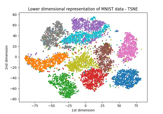
It is clear that data points are separated as clusters according to their class labels. The nearby data points of the same class in the original dimension will still be nearby in the lower dimension!
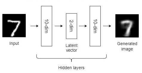
Now, we will use the following autoencoder with only two hidden layers to visualize MNIST data in a lower-dimensional form.
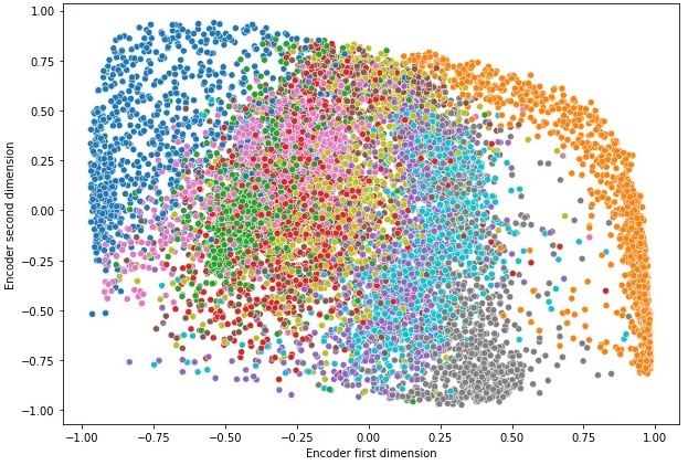
This autoencoder architecture is capable of distinguishing between the nine clusters to some extent, but not perfectly as in t-SNE. The cluster separation is not good enough.
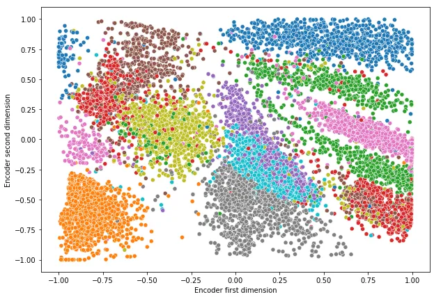
After we increase the number of hidden layers and nodes in the autoencoder architecture as in the following figure, the cluster separation becomes very clear!
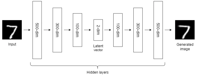
The separation of clusters is very clear now as in t-SNE!
This is the end of today’s article.
Please let me know if you’ve any questions or feedback.
Other dimensionality reduction methods you might be interested in
- Principal Component Analysis (PCA)
- Factor Analysis (FA)
- Linear Discriminant Analysis (LDA)
- Non-Negative Matrix Factorization (NMF)
- Autoencoders (AEs)
- Kernel PCA
- Recursive Feature Elimination (RFE)
- Truncated SVD
- t-SNE
Read next (Recommended)
How about an AI course?
Support me as a writer
I hope you enjoyed reading this article. If you’d like to support me as a writer, kindly consider signing up for a membership to get unlimited access to Medium. It only costs $5 per month and I will receive a portion of your membership fee.
Join my private list of emails
Never miss a great story from me again. By subscribing to my email list, you will directly receive my stories as soon as I publish them.
Thank you so much for your continuous support! See you in the next article. Happy learning to everyone!
Designed and written by: Rukshan Pramoditha
2023–06–30