
Deep Learning | Python HandsOn
AutoEncoders for Land Cover Classification of Hyperspectral Images — Part -1
A walkthrough on utilizing AutoEncoders for land cover classification of Hyperspectral Images using Python.

Dimensionality reduction has become an important aspect of machine learning. It is often considered as a preprocessing step in the machine learning problems such as classification and clustering. The presence of a large number of features in data sets affects the predictive capabilities of the classifiers. The feature extraction algorithms reduce the dimensionality of the data set, thereby paving way for the classifiers to generate comprehensive models at a reduced computational cost.
This article helps readers to understand the role of AutoEncoders in Dimensionality Reduction of Hyperspectral Images and also provides a hands-on tutorial of the implementation.
Table of Contents
- Introduction
- AutoEncoders
- Implementation of AutoEncoder
- Conclusion
- References
Let’s get started ✨
Introduction
The data which we use to develop a Machine Learning model may have replicated or unwanted features, when we deal with real problems we often encounter high dimensional data which may lead to redundant features or over-fitting of the model and it will be a difficult task to visualize the data. So we disrate some of the dimensions in the feature set using Dimensionality Reduction techniques.
Dimensionality Reduction is a statistical technique that is used for converting a set of data having vast dimensions into data with lesser dimensions with the essence that it should provide similar information as of data with the original dimensions concisely without further loss of information in data. Dimensionality reduction can reduce the time that is required to train the Machine Learning model and it can also benefit in the elimination of over-fitting. Dimensionality Reduction approaches can be divided as follows:
- Feature Selection
- Feature Extraction
Feature Selection is the process where you automatically or manually select the most significant features which contribute most to your prediction variable or output in which you are interested. The Feature Selection problem is to find a subset that maximizes the learner's/ ML Model’s ability to classify patterns. Some of the feature selection techniques are Filter Method, Wrapper Method, Hybrid Method, and Embedded Method.
Feature Extraction is a process of dimensionality reduction by which an initial set of input data is reduced to more manageable groups for processing. A characteristic of these large data sets is a large number of variables that require a lot of computing resources to process. Feature extraction is the name for methods that select and/or combine variables into features, effectively reducing the amount of data that must be processed, while still accurately and completely describing the dataset without loss of information. Some of the feature extraction techniques are Principal Component Analysis (PCA), Kernel PCA, IsoMap, Local Linear Embedding (LLE), t-Stochastic Neighborhood Embedding (t-SNE), AutoEncoders, e.t.c.
AutoEncoder
AutoEncoder is an unsupervised dimensionality reduction technique in which we make use of neural networks for the task of Representation Learning. Representation learning is learning representations of input data by transforming it, which makes it easier to perform a task like classification or Clustering.
An Auto-encoder provides a representation of each layer as the output. This network has a tight bottleneck of a few neurons in the middle, driving to create efficient representations that compress the input into a low-dimensional space that can be used by the decoder to reconstruct the original input. A highly fine-tuned autoencoder model should be able to reconstruct the same input in the output layer which was provided in the input layer.
The architecture of an auto-encoder typically contains four main components:
- Encoder: The encoder is a layer in which the input data is provided to the neural network. The encoder comprises a series of layers with a decreasing number of nodes. In this layer, the model learns how to represent the input data by reducing the input data into latent view representation. It can be represented by an encoding function where x is input data.
- Latent View Representation: Latent view represents the lowest possible dimensional space of input data in which the inputs are reduced and information is preserved. It decides which features of data are highly significant and relevant, and the less significant features can be eliminated.
- Decoder: The decoder is similar to that of the encoder but in this case the number of nodes in each layer increases and outputs an almost similar output. In this layer, the model learns how to reconstruct the input from the latent space representation.
- Reconstruction Loss/Error: The reconstruction error measures how different the reconstructed data is from the original data. We should minimize the reconstruction loss by adjusting the parameters in the encoder and decoder.
Implementation of AutoEncoder
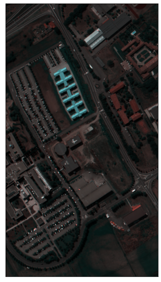
We are going to use Keras to build the autoencoder and the Pavia University Hyperspectral Image data is used to train the autoencoder. The Pavia University HSI was acquired by the ROSIS sensor during a flight campaign over Pavia, northern Italy. The HSI data is publicly available on Group De Inteligencia Computacional (GIC). The Composite Image of Pavia University is shown below.
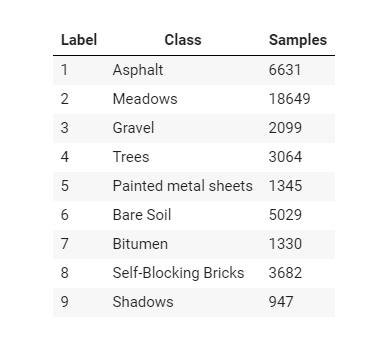
The Pavia university HSI has 103 spectral bands, and It contains 610 * 340 pixels, but spectral samples of the image contain no information which is defined as Zero (0), and they have to be discarded before the analysis. The geometric resolution is 1.3 meters. The groundtruth of the HSI is differentiated into 9 classes. The information of the ground truth is shown in the below image.
Import Libraries
Let’s import the necessary libraries to build and train the autoencoder.
Load data
Usually, this type of data is in the form of .mat files. so we need to read the data and convert it into a pandas data frame for further process.
Visualize Data
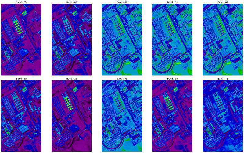
Let’s see a few spectral bands of the Pavia University HSI, the below code randomly plots 10 out of 103 spectral bands of the data.
The output of the above code is shown below:
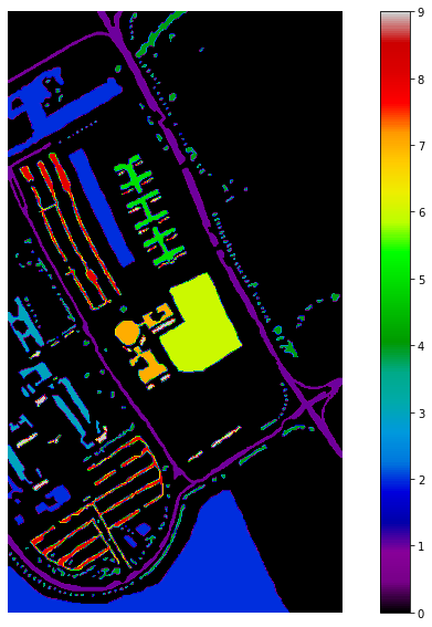
Let’s visualize the ground truth of the Pavia University HSI data, the black color represents the pixels with no information which will be discarded during the classification process.
The output of the above code is shown below:
Build AutoEncoder
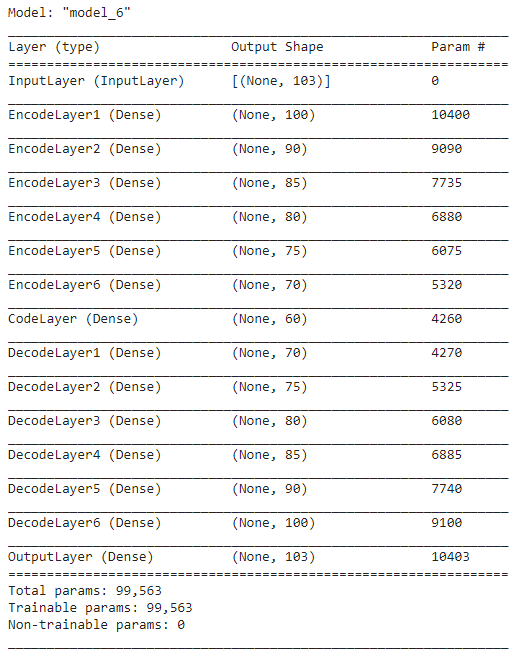
The below code builds the autoencoder which encodes the spectra of the Pavia University HSI with the dimension of 1 * 103 into 1 * 60.
The summary of the autoencoder is shown below:
Training AutoEncoder
For training the defined autoencoder, I have used Adam optimizer, Mean Squared Error(MSE), and Mean Squared Logarithmic Error (MSLE) a loss metric. I have used Early Stopping, Model Checkpoint, and Tensorboard callbacks to tune the model. The below code is used to compile and train the model.
The below graph shows the details of the training loss and MSLE. The x-axis and y-axis represent epochs and loss.
Encode data
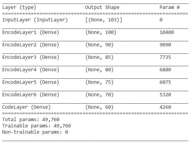
After training the autoencoder, separate the encoder part and feed the data which results in the latent space representation of the original data. The below code servers the above-mentioned purpose.
The summary of the encoder is shown below:
The below code shows how to pass the data, add the class labels for classification tasks, and save the latent space representation of the data into a CSV file.
The first five rows of the reduced data are shown below:
Conclusion
This article shows how to use autoencoders for dimensionality reduction which is further used for land cover classification of Hyperspectral Images. It also helps readers to go through the hands-on tutorial for implementation of autoencoder using python.
The part-2 of the article focuses on the land cover classification of the Hyperspectral Images using the data which is generated by the autoencoder in this article.
Happy Learning!


