Are These Data ‘Normal’? Anomalies & Outliers In Machine Learning

A deep dive into isolation forests with Python

Calculus jokes are mostly derivative, trigonometry jokes are too graphic, algebra jokes are usually formulaic, and arithmetic jokes are pretty basic.

But the occasional statistics joke is an outlier.

Nobody wants outliers in their data — especially when they have come from the likes of false entries due to fat thumbs. A couple of zeros can throw off an algorithm and can destroy summary statistics.

So this is how you use machine learning to remove those pesky outliers.

What is normal?

Historically, the first step to anomaly detection is to try and understand what’s “normal”, and then find examples of “not normal”. These “not normal” points are what we would classify as outliers — they didn’t fit our expected distribution even at the furthest ends of it.

Isolation Forests, or iForest, an elegant and beautiful idea, don’t follow this approach. The premise behind it is simple. The original authors and inventors of the idea for iForests stated that outliers, or anomalies, are data points that are “few and different” from the rest of the population.

They furthered by noting that data points that are “few and different” suffer from a characteristic called “isolation”.

Seems logical.

How does it work?

The isolation forest algorithm works by isolating instances without relying on any distance measure. They use a combination of the two features they prescribed to anomalies earlier — that anomalies are both few and different.

The algorithm makes use of binary tree structures. Which are recursive structures that have at most two children resulting from each node.

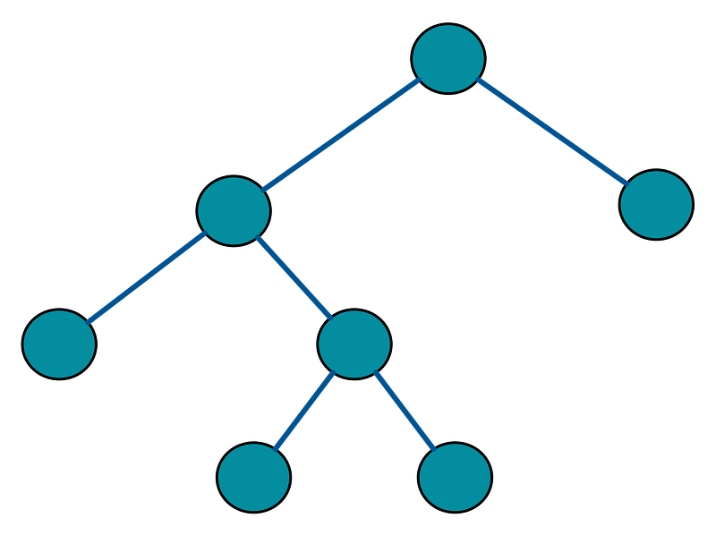
Here’s the important bit.

Because of their susceptibility to being isolated, outliers are more likely to be located near the ROOT of the tree — it takes fewer partitions to isolate them.

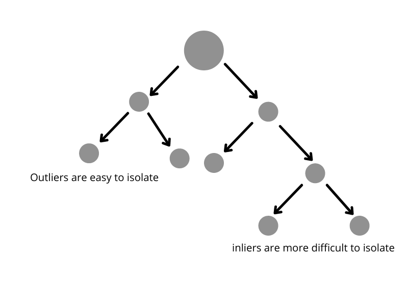
Therefore, points with a shorter path length are likely to be outliers. The iForest algorithm builds an ensemble of iTrees (seem familiar?) and then averages the path length.

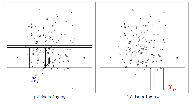
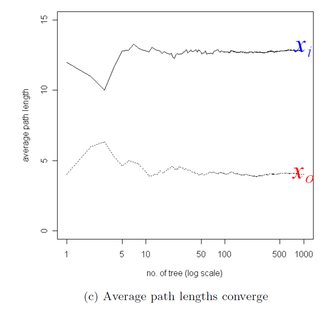
As you can see from the original author's images above, the point our eye clearly tells us is an outlier takes much less partitioning to be isolated. The path length converges at less than half the length of the point which is clearly not an outlier.

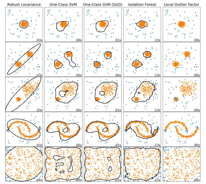
How does it compare to other anomaly detection algorithms?

Firstly, there are a lot of benefits to using iForest. Here are some examples.

• iForest can exploit sub-sampling so it has a low linear time complexity and a small memory requirement.
• It can deal with the effects of swamping and masking.
• Works well on high dimensional problems.
• Works well with irrelevant attributes.
• Works without training sets that include anomalies (unsupervised).

But the main reason that iForest is so great at what it does is due to the fact that it was designed for this job. This isn’t the case for a lot of its counterparts. Algorithms such as one-class SVM and most clustering methods are designed for other purposes. They suit anomaly detection but still were not created for this purpose.

A full comparison of different anomaly detection algorithms can be seen here.

From this picture alone I know which one I fancy using.

Here’s how it works in Python

It’s easy to run in Python. As you can see it's only 30 or so lines to get the predictions.

All you have to do is import the packages and your data. Then, convert it to a Numpy array before running and fitting the model. You can then convert it back to a pandas dataframe and run the value_counts method on it and this will tell you how many outliers you have. From the dataset I used, the algorithm picked up 148 outliers — which it then assigns the value of -1.

You can then merge this back onto your original dataframe and use your plotting package of choice to have a look at the outliers it has predicted.

I hope this all makes sense and happy (outlier) hunting.

Cheers,

James

If I’ve inspired you to join medium I would be really grateful if you did it through this link — it will help to support me to write better content in the future.

If you want to learn more about data science, become a certified data scientist, or land a job in data science, then checkout 365 data science through my affiliate link.

If you enjoyed this, here are some more of my articles.