Applying Statistics in Python — Part III

Multiple Linear Regression, R², Adjusted R², MSE, p-value

Here’s the Friend Link to read this member-only story.

Statistics and coding are fundamentally important in the data science field. Since a lot of a data science work is carried out with code, I would highly recommend learning statistics with a heavy focus on coding, preferably in Python or R.

In my previous article, I shared about how to code summary statistics (Mean, Median, Mode, Max, Min, Range, Quartile, Inter-Quartile Range, Standard Deviation, Variance) of a dataset and the Simple Linear Regression.

In this article, I shall cover the following topics with codes in Python 3: • multiple linear regression models • model performance metrics: R², Adjusted R², MSE, p-value

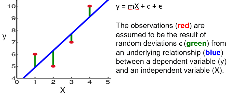
Recap: Linear Regression is the practice of statistically calculating a straight line that demonstrated a relationship between two different items. A linear relationship can be positive or negative. A Simple Linear Regression is a statistical model that relates the linear relationship between two variables: 1 dependent and 1 independent variable. For example: y = mX + c + ϵ

Multiple linear regression models

Recap: A Multiple Linear Regression is a statistical model that relates the linear relationship between three or more variables: 1 dependent variable and 2 or more independent variables. For example: y = β0+ β1X1 + β2X2 + β3X3 + βnXn + ϵ

where ϵ is the model’s random error (residual) term.

Multiple linear regression is based on the following assumptions: · A linear relationship between the dependent and independent variables · The dependent variables are not highly correlated with each other · The observations are independent of one another · The residuals are normally distributed (multivariate normality) · The variance of the residuals is constant (homoscedasticity)

Multiple linear regression models also capture the errors in the data, also known as residuals. Residuals are the differences between the true value of y and the predicted (or estimated) value of y. In a regression model, we are trying to minimize these errors by finding the “goodness of fit” — the regression line of best fit where errors would be minimal.

There are two main ways to perform linear regression in Python — with Statsmodels and Scikit-learn. Reading the data set from my GitHub to predict the dependable variable ‘Life Expectancy’ as ‘y’, using various independent variables in the ‘X’ DataFrame.

(i) Regression using Statsmodels Since the linear regression model minimizes the squared error the solution is referred to as the least squares solution.

import pandas as pd
import statsmodels.api as sm

df = pd.read_csv('df3.csv')
# slice data into features X and target y
X = df[ ['Birth Rate', 'Cancer Rate', 'Dengue Cases',
         'EPI', 'GDP', 'Health Expenditure',
         'Heart Disease Rate', 'Population', 'Area',
         'Pop Density', 'Stroke Rate'] ].astype(float)
X = sm.add_constant(X)
y = df['Life Expectancy']

# Baseline results
model = sm.OLS(y, X)
results = model.fit()
results.summary()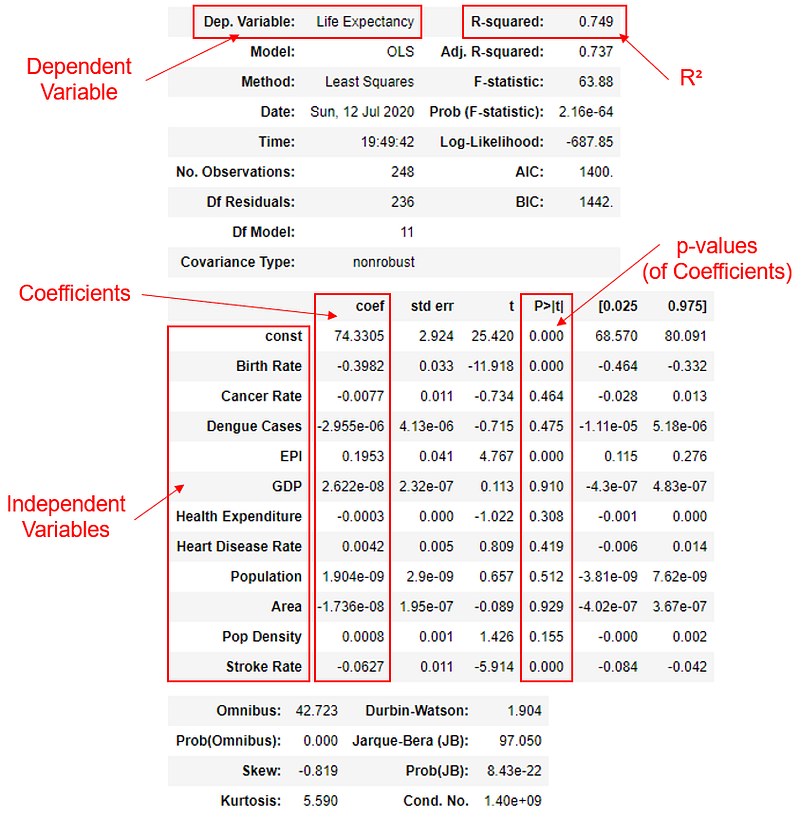

(ii) Regression using Scikit-learn Scikit-learn fits a linear model with coefficients β = (β1, …, βn) to minimize the residual sum of squares between the observed targets in the dataset, and the targets predicted by the linear approximation.

import pandas as pd
from sklearn.linear_model import LinearRegression

df = pd.read_csv('df3.csv')
# slice data into features X and target y
X = df[ ['Birth Rate', 'Cancer Rate', 'Dengue Cases',
         'EPI', 'GDP', 'Health Expenditure',
         'Heart Disease Rate', 'Population', 'Area',
         'Pop Density', 'Stroke Rate'] ].astype(float)
y = df['Life Expectancy']

# Fit the model to the full dataset
model = LinearRegression()
model.fit(X, y)
# Print out the R^2 for the model against the full dataset
print(model.score(X, y))
# print out intercept
print(model.intercept_)
# print out other coefficients
print(model.coef_)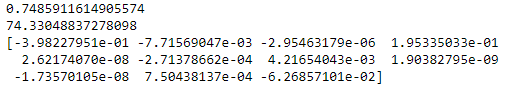

Which method should I use?

(i) Statsmodels is rather straight forward, with all outputs displayed neatly in a table. Feature selection can be done by looking at the p-value. For example, when p-value < 0.05, the coefficient is significant, and the corresponding variable is a significant variable in the model.

(ii) SkLearn can do more with (train-test split) cross validation to have a more robust way to determine R² value or other loss functions. Feature selection is done using Lasso L1 regularization. I personally prefer to use this method, as the library can also be extended to other machine learning applications like classification, for examle, predicting employee attrition.

R² value — how well the model fits the data

The R² value, also called the coefficient of determination, states the proportion of variability in the data set that is explained by the model.

from sklearn.metrics import r2_score

r2 = r2_score(y, model.predict(X))
# 0.7486

It measures the “goodness of fit” and the proportion of variability around the mean explained by the model. It is a value ranging from 0 to 1, with 0 stating that the model has no ability to make prediction, and 1 stating that the model predicts the result perfectly.

Adding independent variables to a multiple linear regression model will always increase the amount of explained variance (i.e. R²) in the dependent variable. Therefore, adding too many independent variables without any theoretical justification may result in an over-fit model (with high R²).

Adjusted R² measures the same as R² (variability explained by the model), but taking into consideration the number of independent variables. Increasing the number of independent variables will result in a decrease in Adjusted R². Adjusted R² is always smaller than the R² value, as it penalizes excessive use of variables.

Mean Squared Error (MSE)

In statistics, the MSE of an estimator (or statistical model) measures the average of the squares of the errors — that is, the average squared difference between the estimated values and what is estimated. MSE is a risk function, corresponding to the expected value of the squared error loss.

Root Mean Squared Error (RMSE) is just the square root of MSE. This value on its own is meaningless. It needs to be compared with the RMSE of another model to make comparisons, to see which model is better (lower the better).

import numpy as np
from sklearn.metrics import mean_squared_error

# root mean squared error
rmse = np.sqrt(mean_squared_error(y, model.predict(X)))
# 5812.0

The goal of the model is to minimize the squared errors as much as possible. The best estimate for the model’s parameters is the principle of least squares, which is a measure of how observations deviate from the regression line.

What is the p-value?

I define the null hypothesis as the original state at status quo, without changing any variable. This null hypothesis is true until I have evidence that it is not. I then gather a random sample and calculate its test statistics.

The p-value is the probability of getting this random sample I gathered (or more extreme than this) if the null hypothesis is true. It describes how remotely possible is the sample obtained. For large p-value, the null hypothesis is highly likely to be true, i.e. it is not surprising to get such a sample if the null hypothesis is true.

As the p-value gets smaller, it becomes more unlikely to obtain such a sample, thus the null hypothesis might perhaps be doubtful and incredible. For a coefficient to be statistically significant, I usually want a p-value of less than 0.05.

Take a break!

Apart from working on data science projects, my other hobby is problem solving on HackerRank to sharpen my skills.

I encourage you to try out 10 Days of Statistics, with solutions compiled here.

Thank you for reading! I hope you have enjoyed reading my stories. To get unlimited access to quality content on Medium, join as a Medium member!