Applying Principal Component Analysis (PCA) create a regression model in R

Before we start, let’s begin with a quick overview of what PCA is and when it is used. Then, we will dive into how to use PCA in R and some of the common ways we can go about selecting the principal components to create a regression model in R.

PCA is primarily used for exploratory data analysis and for making decisions in predictive models. It is also for dimensionality reduction and finding relevant components that account for most of a data’s variability.

To keep it super simple, the steps to carry out PCA are:

1. Center the data
2. Scale the data [optional]
3. Carry out data reduction
4. Undo any scaling [optional]
5. Undo the centering [optional]

Now that that’s out of the way, I’ll primarily cover how to apply PCA in R to create a regression model. To follow along, I will be using statsci’s dataset uscrime.txt (the file name uscrime.txt with description), along with regression R function lm to predict the observed crime rate in a city. We will also be scaling the data here as well.

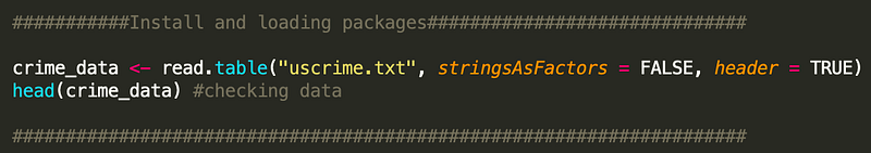
So we start by loading the data in RStudio:

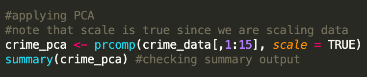
We then apply PCA and set scale = TRUE for scaling the data as part of the PCA function. By specifying scale = TRUE, each of the variables in the dataset are scaled to have a mean of 0 and a standard deviation of 1 before calculating the principal components. From there, PCA transforms the correlated features in the data into linearly independent (orthogonal) components so that all the important information from the data is captured while reducing its dimensionality.

This is important because PCA is sensitive to the scale of the data. If you don’t center and scale the data, features with larger variances will dominate the principal components. If the range of the variables (which, recall, are in the columns) are approximately the same, one generally does not scale the data. However, if some variables have much larger ranges, they will dominate the PCA results. Also, since we are using “prcomp()”

Lets check the summery output of the PCA results:

Here are some other commands you can try for further epxloration:

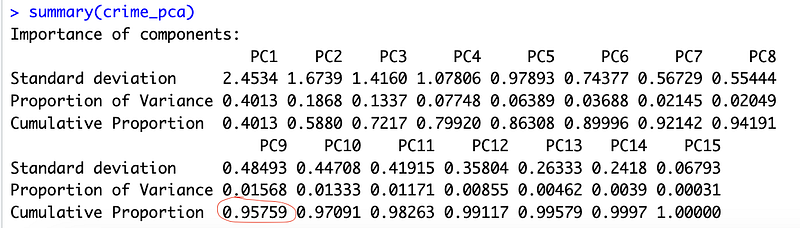
Before diving too deeply into the above output, let me give a quick summary eigenvectors. Eigenvectors are unit vectors with length or magnitude equal to 1. They are often referred to as right vectors, which simply means a column vector. Eigenvalues are coefficients applied to eigenvectors that give the vectors their length or magnitude. As we have 15 predictors here (or principal components as seen listen PC1 — PC15 above), we get 15 eigenvalues.

Now, notice above that I have circled 0.95759 in red. What does that cumulative proportion mean? Let’s start with the first cumulative proportion we see under PC1 (0.4013). The first principal components explain the the variability around 40%. Notice here that in this case of the one we circled, approximately 95% of the variance can be explained with the first 9 principal components (in other words the first nine components capture the majority of the variability).

We can get a similar view of this by using the “get_eigenvalue()” command:

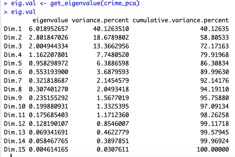
Recall now that we are looking for a cutoff to decide how many princiapl components we want to select for our regression model. To do that here, we are going to be setting the eigenvalue > 1. This is the “classical” cutoff value for eigenvalues since the eigenvalue is a measure of the information value of a factor, scaled in variables; according to that, an eigenvalue of less than one is less efficient in terms of information than the average single variable. This holds true only when the data are standardized. Unfortunately, there is no well-accepted objective way to decide how many principal components are enough. In our analysis, the first five principal components explain 86.3% of the variation. This is an acceptably large percentage.

Just to further validate, we also use an alternative method to determine the number of principal components by looking at a Scree Plot, which is the plot of eigenvalues ordered from largest to the smallest. The number of component is determined at the point, beyond which the remaining eigenvalues are all relatively small and of comparable size.

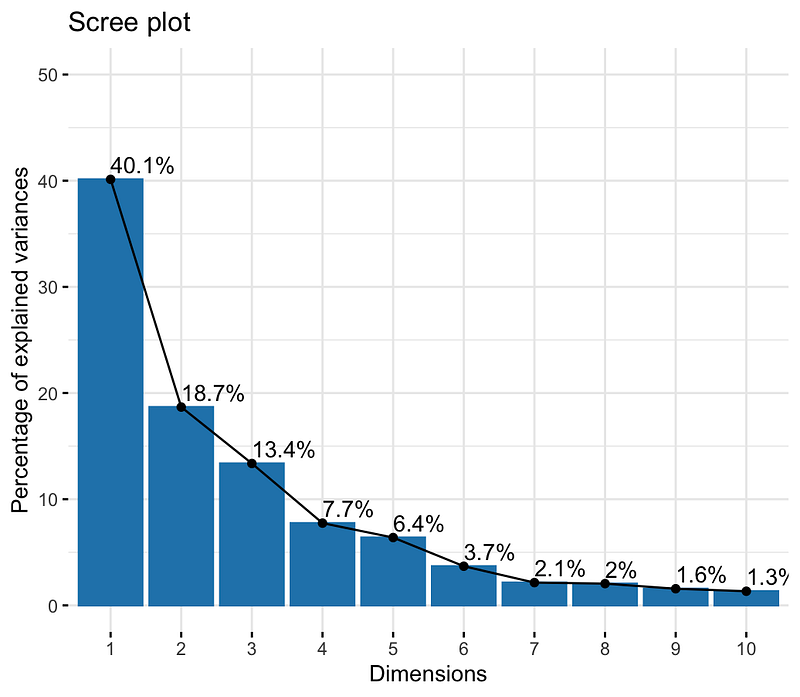
From the plot above, we see again that we might want to stop at the fifth principal component. 86.3% of the information (variances) contained in the data are retained by the first five principal components.

Now, that we’ve identified this, let’s use the first 5 principal components to create a regression model.

To follow along with how to apply these principal components to create a lm regression model, please click on my next blog.