Another Steep Curve? Predicting India’s COVID-19 Third Wave with LSTM

Complete project of predicting new COVID-19 cases in the next 90 days with LSTM (code included)

India is seeing a steep rise in COVID-19 cases again! Only 6,358 new cases were registered on 27 December 2021. But in just 14 days, on 10 January 2022, a whopping 168,063 new cases were registered. The curve of the third wave is very steep and that’s why it is a big concern right now.

So, I thought about using the artificial recurrent neural network (RNN) architecture Long Short-Term Memory (LSTM) to predict how the COVID-19 graph will look in near future (next 90 days).

Dataset:

The dataset is downloaded from ‘COVID-19 India Datasets by DataMeet’. The data is community collected, cleaned and organized from different government websites which are freely available to all the Indians.

Github Repository: https://github.com/datameet/covid19

The dataset has a Creative Commons Attribution 4.0 International Public License. The dataset is downloaded on 10 January 2022 and contains data up to the same date.

We are using the file all_totals.JSON file in the data directory. The pre-processing step demonstrates how I processed the data from this JSON file to use it for the LSTM architecture.

Methodology

Let’s discuss the methodology of how I executed the project. The result sections after this will have a discussion of the results we got from the whole project.

Import Libraries:

Let’s import the necessary libraries for the project.

import json
import numpy as np
import pandas as pd
import matplotlib.pyplot as plt
from sklearn.preprocessing import MinMaxScaler
from tensorflow.keras.models import Sequential
from tensorflow.keras.layers import LSTM,Activation,Dense,Dropout
%matplotlib inline
scaler = MinMaxScaler()
from tensorflow.keras.callbacks import EarlyStopping

Data Pre-Processing:

From the dataset all_totals.JSON, I created a dataframe that contains new cases registered every day.

f = open('all_totals.json')
# returns JSON object as a dictionary
data = json.load(f)

total_cases_list = []
new_cases_list = []
    
pre_total_cases = 0
for row in data["rows"]:
    if "total_confirmed_cases" in row["key"]:
        temp_list = []
        temp_list.append(row["key"][0][0:10]) # Appending the date (the time part is trimmed)
        temp_list.append(row["value"]) # Appending the value on that date
        total_cases_list.append(temp_list)
        
        temp_list_2 = []
        temp_list_2.append(row["key"][0][0:10])
        temp_list_2.append((row["value"] - pre_total_cases)) # Appending the value on that date
        new_cases_list.append(temp_list_2)
        
        pre_total_cases = row["value"]
    
df_total = pd.DataFrame(total_cases_list, columns = ["Date", "Total Cases"])
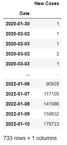
df_new = pd.DataFrame(new_cases_list, columns = ["Date", "New Cases"])

The dataframe named df_new contains new cases registered on each day (some dates are missing), starting from 2020–01–30.

Let’s make the ‘Date’ field the index.

df_total = df_total.set_index("Date")
df_new = df_new.set_index("Date")

Let’s delete some faulty values in the file:

#deleting two faulty values

df_total.drop('2021-09-16', inplace=True, axis=0)
df_total.drop('2021-09-17', inplace=True, axis=0)
df_total.drop('2021-07-21', inplace=True, axis=0)
df_total.drop('2021-07-22', inplace=True, axis=0)

df_new.drop('2021-09-16', inplace=True, axis=0)
df_new.drop('2021-09-17', inplace=True, axis=0)
df_new.drop('2021-07-21', inplace=True, axis=0)
df_new.drop('2021-07-22', inplace=True, axis=0)

This is how the dataframe looks now:

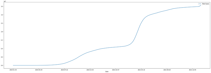
Let’s see the curve of total cases of COVID-19 registered in India:

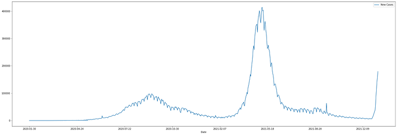
And this is the curve of new cases of COVID-19 registered in India:

Now we will build the training dataset and training labels. The training dataset will be time-series data. We chose 90 days as the window size of the time series data.

day = 90 # Number of days (window size)

Let’s create the training dataset and training labels now.

k = 0

array = []
array_temp = []
train_data = []
train_labels = []

for i in range(len(df_new)):
    array_temp.append(df_new.iloc[i]['New Cases'])

array_temp = np.array(array_temp).reshape(-1,1)
array_temp = scaler.fit_transform(array_temp)
array_temp = array_temp.tolist()

for i in array_temp:
    array.append(i[0])

for i in range(len(array)):
    try:
        train_data.append(array[k:day+k]) # Creating inner lists with 'day' days of data
        train_labels.append([array[day+k]])
        k+=1
    except:
        break

length = max(map(len, train_data))
train_data=np.array([xi+[None]*(length-len(xi)) for xi in train_data]).astype('float32')

length = max(map(len, train_labels))
train_labels = np.array([xi+[None]*(length-len(xi)) for xi in train_labels]).astype('float32')

We used the MinMaxScaler to bring our data in the 0–1 range. Then we reshaped it to make it just one column and n number of rows (n = number of elements in the array). After that, we converted the array to a list.

Then, we created the training data. For every 90 points in one list, the 91st point will be the label of them. Then we created a list of lists with all the lists containing 90 points. We created another list containing the labels. Later, all those lists are converted into NumPy arrays and NumPy arrays or arrays.

The Shape of the training and the label dataset is like this:

print(train_data.shape)
print(train_labels.shape)

Shape:

(644, 90) (643, 1)

Let’s expand the dimensions of the training dataset for the LSTM architecture.

train_data = train_data[:len(train_labels)]
train_data = np.expand_dims(train_data,1)
train_data.shape

Shape: (643, 1, 90)

Let’s see how one row of the training data looks now.

train_data[1]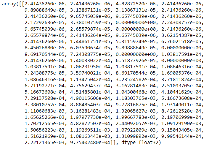

Let’s see how one row of the label dataset:

train_labels[1]

Output: array([0.0027741], dtype=float32)

Architecture:

Let’s build the LSTM architecture now

model = Sequential()

model.add(LSTM(250,input_shape=(1,day)))
model.add(Dropout(0.5))

model.add(Dense(250,activation='relu'))
model.add(Dropout(0.5))

model.add(Dense(day,activation='relu'))
model.add(Dropout(0.5))

model.add(Dense(1,activation='relu'))

model.compile(loss='mean_squared_error',optimizer='adam')

model.summary()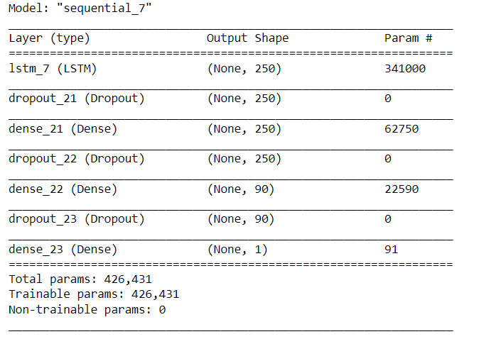

Training:

The fit the data to the model now.

E = 1000
callback = EarlyStopping(monitor='loss', mode='min', patience=20)
H = model.fit(train_data,train_labels,epochs=E, verbose=0, callbacks=[callback])

After the training step is done, let’s plot the loss value.

loss = H.history['loss']
epochs = range(0,len(loss))
plt.figure(figsize=(15,5))
plt.plot(epochs,loss)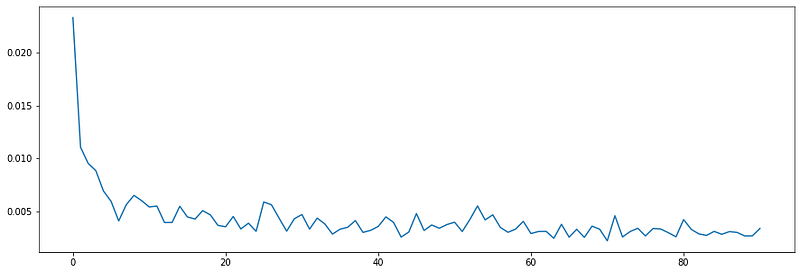

Let’s plot the predictions given by LSTM along with the real values of newly registered COVID-19 cases each day to see how accurate the predictions are.

preds = scaler.inverse_transform(model.predict(train_data))
plt.figure(figsize=(30,10))
plt.plot(preds,label='our predictions')
plt.plot(scaler.inverse_transform(train_labels),label='real values')
plt.legend()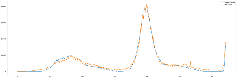

From this graph, we can see that the predicted values are very accurate and the model is very promising.

Future Predictions:

Let’s try to predict this curve in the near future. We will try to predict how many cases new cases of COVID-19 will be registered in India for the next 90 days (starting from 10 January 2022).

days_to_predict = 90
seed = array[-day:]
#seed

What we are doing here is, we are creating a seed. A seed is nothing but the last 90 days of data in the array. We will use this seed to predict the data for the next day. When it will predict it then we will update our seed, and make it contain the predicted data to be used in the next prediction.

Let’s take an example. The seed first contains the last 90 days of data (values of how many new covid cases are registered each day), ending on January 10, 2022. Using it, we will predict the value for 11 January 2021. Then we will use the predicted data of 11 January 2022 as a datapoint in the seed and predict the value data for 12 January 2022 and so on.

Let’s use this model to predict the number of cases for the next 90 days:

for _ in range(days_to_predict):
    current_days = seed[-day:]
    current_days = np.squeeze(current_days)
    current_days = np.expand_dims(current_days,0)
    current_days = np.expand_dims(current_days,0)
    pred = model.predict(current_days)
    seed = np.append(seed,pred)

Let’s plot the predicted values:

upcoming_days_prediction = scaler.inverse_transform(seed[-days_to_predict:].reshape(-1,1))
plt.figure(figsize=(30,10))
plt.plot(range(0,days_to_predict),upcoming_days_prediction)

Let’s add the predicted values with the values in our dataset and plot the complete graph.

# Adding real values and predicted values together
arr_without_pred = scaler.inverse_transform(train_labels)
arr_pred = scaler.inverse_transform(seed[-days_to_predict:].reshape(-1,1))
arr_with_pred = np.concatenate((arr_without_pred, arr_pred))

plt.figure(figsize=(30,10))
plt.plot(arr_with_pred)

Results:

Before we see the results, I hope you are enjoying reading this article. If you did, please become a member of Medium. Just for 5$ per month, you can read any article on Medium (not just my articles, any article). Click the link below.

https://samratduttaofficial.medium.com/membership

I will get a small commission from the 5$ and it will motivate me to write more!

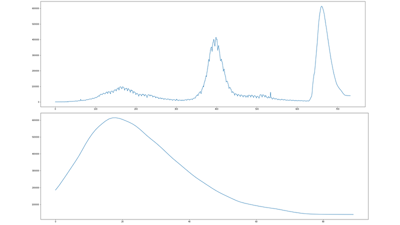
Let’s see the prediction of newly registered COVID-19 cases for the upcoming 90 days (starting from 11 January 2022).

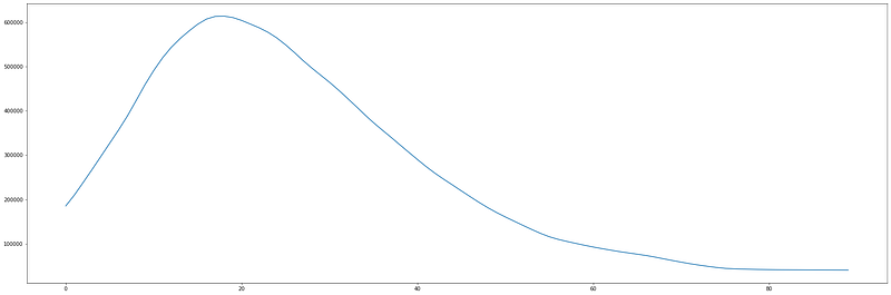
Let’s see the complete graph of newly registered COVID-19 cases each day, along with the predicted values for the upcoming 90 days (starting from 11 January 2022).

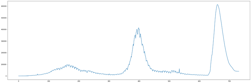
So, how many total cases does the model predict for the upcoming 90 days?

total_new_cases = 0
for i in upcoming_days_prediction:
    total_new_cases += i[0]
    #print(i)
print(total_new_cases)

The answer is: 23,417,088

This model predicts about 23.5 million new COVID-19 cases in India in the upcoming 90 days (starting from 11 January 2022).

Conclusion

This study/project just showcases the usage of the LSTM architecture in predicting time-series data. In this case, we used the COVID-19 data from India for our study. This model does not consider transmissibility and other factors while making the predictions.

Since the transmissibility of the Omicron variant is much higher than the Delta variant of COVID-19 (the Delta variant was the dominant variant during the second wave of the pandemic in India), I personally think that we will see a much steeper and higher curve in the near future.

But I am no health worker or doctor. So take everything I say with a grain of salt.

Repository: https://github.com/SamratDuttaOfficial/Covid_India_LSTM

Make sure to give the Github repository a star.

Samrat Dutta:

Github: https://github.com/SamratDuttaOfficial

Linkedin: https://www.linkedin.com/in/SamratDuttaOfficial [Hire Me]

Wisest Friends (Machine Learning) Discord: https://discord.gg/7Bx6PGVy

Buy me a coffee: https://www.buymeacoffee.com/SamratDutta