Summary

This article discusses the use of Fourier transforms in Python with SciPy to analyze seasonality in 911 phone call data from Montgomery County, PA, aiming to identify patterns that can inform staffing decisions for the call center.

Abstract

The article titled "Analyzing seasonality with Fourier transforms using Python & SciPy" provides a practical guide on how to separate signal from noise in time series data, specifically focusing on 911 phone call records. It introduces the Fourier transform as a tool to identify seasonal trends in the data, such as variations in call volume throughout the day, week, or year. By analyzing the frequency components of the call data, the article demonstrates how to detect significant seasonal patterns, which can be crucial for optimizing staffing levels in the 911 call center. The author emphasizes the importance of data preparation, including aggregating call counts at appropriate time intervals and handling missing data. The use of the Fast Fourier Transform (FFT) algorithm from the scipy.fft submodule is highlighted for its efficiency in computing the transform. The article also addresses the challenges of interpreting the results, such as dealing with aliasing and identifying the most relevant frequencies. It concludes with a discussion on the limitations of using Fourier analysis alone for precise timing of seasonal spikes and suggests incorporating Fourier terms into regression models for more accurate predictions.

Opinions

The author believes that understanding seasonal patterns in data can lead to smarter decision-making.
Fourier transforms are presented as an effective method for separating signal from noise, particularly in identifying underlying frequencies that contribute to the signal.
The article suggests that real-world data often contains noise, and the Fourier transform is a valuable technique for revealing the true signal.
The author recommends a practical approach to learning about Fourier transforms, starting with a hands-on exercise before delving into the mathematical derivations.
The concept of the Nyquist rate is emphasized as a rule of thumb for sampling frequency to avoid aliasing.
The author posits that the Fast Fourier Transform (FFT) is the standard method for computing Fourier transforms due to its efficiency, akin to Quicksort in sorting algorithms.
The article points out that while Fourier analysis can identify seasonal patterns, it may not pinpoint the exact timing of these patterns without additional analysis, such as incorporating the results into regression models.
The author's opinion is that combining Fourier analysis with regression models can enhance the prediction of future trends by explaining residuals and combining seasonality with other variables.

Analyzing seasonality with Fourier transforms using Python & SciPy

Learn to separate signal from noise by looking for seasonal trends in 911 phone call data

By the end, you’ll be able to do this with your own data

Analyzing 911 phone call seasonality

As the saying goes, history repeats itself. Understanding these patterns helps us make smarter and more prepared decisions. The challenge is separating the pattern from the noise surrounding it. We can use the Fourier transform, commonly used by engineers, to accomplish exactly that—separate signal from noise.

Today, let’s analyze 911 phone call data from Montgomery County, PA. We’re looking to answer whether there are higher or lower levels of 911 calls during:

Certain hours of the day?
Certain days of the week?
Certain months of the year?

Based on the results, we can make decisions on how to staff our 911 call center. For example, if we find that call volume is highest on Friday evenings, we can offer more shifts on Friday evenings so our call center can handle the higher call volume.

What does the Fourier transform do?

The Fourier transform allows you to transform a function of time and signal into a function of frequency and power. This tells you what frequencies make up your signal and how strong they are. In our case, the signal is the number of phone calls and we might be expecting some kind of weekly or daily frequencies.

On the left, we graphed the sum of two sin waves, one with a period of 5 and frequency of 1/5=0.2 and the other with a frequency of 1/10=0.1. In the Fourier transform, we can clearly see that we have two waves with frequencies of 0.2 and 0.1 by looking at the frequencies corresponding to the peaks.

Real data often contains noise and the Fourier transform lets us see through the noise, and see which frequencies actually matter.

We took the signal from before and added random noise, and we can still clearly see the same frequencies of the signal in the Fourier transform. This is how the Fourier transform separates signal from noise.

This article won’t delve into the mathematics and derivation of Fourier transform here. If you’re interested, I recommend watching 3Blue1Brown’s Visual Introduction to the Fourier Transform after completing this exercise. I recommend doing this exercise first because Fourier Transforms are one of those concepts where starting with a practical example will help you appreciate the mathematics behind it.

Data preparation

First, let’s import and prep the call data. To follow along, you can clone this Github repo and follow the instructions there. The code is here. The raw data is from Kaggle.

For the data prep, let’s transforming the raw data to count the number of calls each hour. We’re aggregating call count at the hour level because call volume at the minute-level is too low and we’re not expecting to see any seasonality below the hour-level. As a rule of thumb, you want your sampling frequency to be twice the highest component frequency you’re expecting to find in the signal. If your frequency is any lower, a condition called aliasing occurs and distorts your results. The minimum frequency where you meet the “2× highest component frequency” rule is referred to as the Nyquist rate. Intuitively, this concept makes sense because we can’t count phone calls per day to answer how the hour of the day impacts phone call volume.

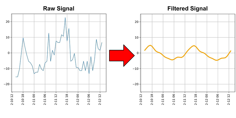
Also, we need to make sure we fill in any missing hours (where there were no 911 calls) with zeros. Finally, for the signal, let’s chart the difference from the average call count instead of the call count itself. This way, our data is centered around 0, like a real sine wave.

The first week of data is plotted on the right. Definitely seeing some seasonality here, so it looks like our analysis will be promising.

Fourier transform

We’ll be using the Fourier Transforms submodule in the SciPy package—scipy.fft. We’ll be using the SciPy Fast Fourier Transform (scipy.fft.fft) function to compute the Fourier Transform. If you’re familiar with sorting algorithms, think of the Fast Fourier Transform (FFT) as the Quicksort of Fourier Transforms. FFT is a more efficient way to compute the Fourier Transform and it’s the standard in most packages.

Just pass your input data into the function and it’ll output the results of the transform. For the amplitude, take the absolute value of the results. To get the corresponding frequency, we use scipy.fft.fftfreq. We can chart the amplitude vs. the frequency. The frequencies with the highest amplitude are indicative of seasonal patterns. Frequencies with low amplitude are noise. Also, scipy’s periodogram function can also get you to a similar chart. Let’s mark the frequencies where we clearly see spikes in amplitude.

If we look at those frequencies with the highest amplitudes and convert them into hours and days, we see that the top seasonal pattern has a daily frequency (the period is ~1 day).

After that, the amplitude sharply drops off and we see seasonality at 8 hours and 7 days. The former suggests there’s a spike in call volume 3 times a day (potentially morning, evening, and late-night?). The latter suggests that call volume spikes one day out of the week.

The other frequencies are difficult to contextualize, but they’re not very important given their low amplitudes.

Inverse Fourier transform

Our analysis isn’t too actionable so far. We know there’s daily seasonality, but don’t know what time of day actually has higher seasonality. To figure this out, we can use the inverse Fourier transform. In theory, this should let us convert our filtered results and view just the signal.

Here’s what that looks like if we chart the filtered signal over the original signal for the first 5 days of data.

Looks promising! The peaks in the filtered signal line up with the original signal around 5 pm. The problem is that when we stretch this out to the last week of data, the peaks start occurring at 11 am instead.

So what gives? The problem is that our frequency wasn’t exactly once every 24 hours. It was actually once every 23.996 hours, and over the course of the entire dataset, that small deviation adds up.

What can we do?

So we’ve answered our initial questions around what kind of seasonality is in the data, but we haven’t been able to answer when seasonality spikes accurately. To take our analysis to the next level, we need to incorporate seasonality into our regression models.

This will help us figure out when seasonality spikes by trying different inputs inspired by our Fourier results. Additionally, this will allow us to combine seasonality with other variables in our regression model so we can predict future call volume more accurately. We’ll also see how seasonality is often used as a way to explain the residuals in a regression model.

To learn more about analyzing seasonality, check out the article linked below, where I go over how to use Fourier analysis in your regression models.

How to add Fourier terms to your regression & seasonality analysis (using Python & SciPy)

Include seasonality in your regressions by using Fourier terms

towardsdatascience.com