
Analysis of Tweets on the Hong Kong Protest Movement 2019 with Python
Disclaimer: This article is not intended to make any form of political or social commentary whatsoever on the current situation in Hong Kong. The analysis done is purely based on deductions made of the data set at hand.
I was motivated to do a pet project on Sentiment Analysis after completing a Deep Learning Course on Coursera taught by Andrew Ng recently, where one of the specialisations is on Sequence Models. I wrote this article to consolidate and share my learning and codes.
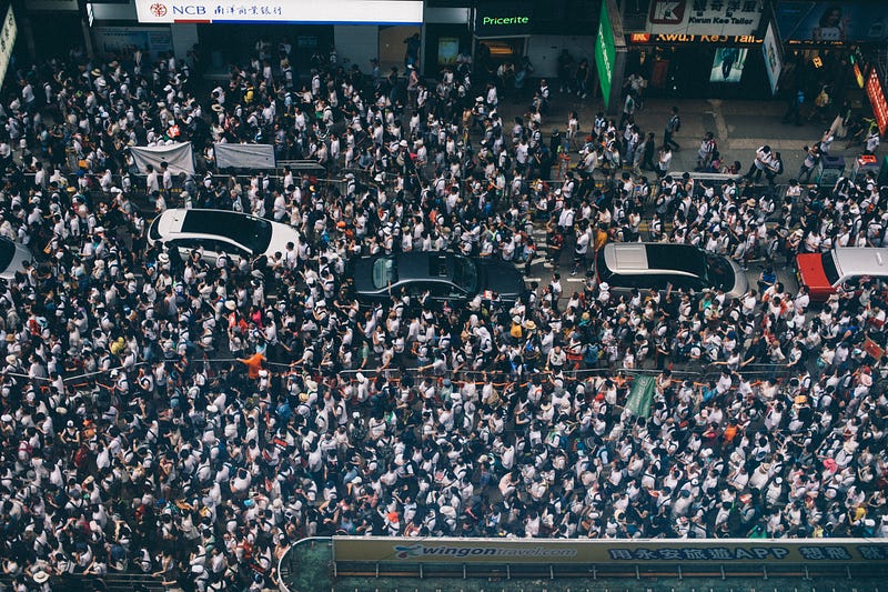
With the Hong Kong protest movement already happening for close to 6 months, I had the sudden idea of scraping Twitter tweets about the protests and using them for this project. I did not want to use existing (and possibly already cleaned up) data sets that are easily available on Kaggle, for instance. I figured this was the chance for me to get my hands dirty and learn the process of scraping the tweets.
The aim for this project is to discover the:
- general sentiment of the tweets regarding the protest, in particular, what are these tweets’ stances/opinions towards the central government in China, Hong Kong administration and police force
- demographics of twitter users
- popularity of hashtags
- behaviour of top users and users in general
- daily top tweets
The structure of this article will be different from the usual tutorials, where the flow would be data cleaning and preprocessing, followed by exploratory data analysis and then model training and tuning. Here we want the reader to focus first on the data analysis and visualisation. Data cleaning and preprocessing steps are covered afterwards. You may access the source code from this repository.
Scraping Twitter Tweets using Tweepy
Since scraping Twitter tweets is also not the focus of this article, I have put up a separate article describing in detail the process of scraping. Click on this link, if you need a step by step guide.
Exploratory Data Analysis (EDA)

Let’s explore and visualise the already processed tweets with the usual data visualisation libraries — seaborn and matplotlib.
1. WordCloud — Quick Preview of Popular words found in tweets regarding the protest
First of all, we use a Word Cloud that can immediately show us what are the most heavily used words in tweets pertaining to the protest. The codes are required are as follows:
from wordcloud import WordCloud
import matplotlib.pyplot as plt
def show_wordcloud(data, title = None):
wordcloud = WordCloud(
background_color = 'white',
max_words = 200,
max_font_size = 40,
scale = 3,
random_state = 42
).generate(str(data))fig = plt.figure(1, figsize = (15, 15))
plt.axis('off')
if title:
fig.suptitle(title, fontsize = 20)
fig.subplots_adjust(top = 2.3)plt.imshow(wordcloud)
plt.show()
# print wordcloud
show_wordcloud(data['cleaned_text'])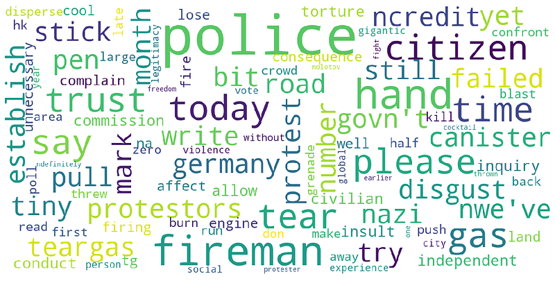
We generated a word cloud for the top 100 words, where the more popular a word is, the bigger the word will be in the word cloud (You can adjust this parameter by changing the value for ‘max_words’).
Some of the words that hit us quickly are: disgust, police, fireman, protestors, tear gas, citizen, failed, trust and etc. In general, without the context of the tweet we cannot determine if each word, taken as its own, represent a negative or positive sentiment towards the government or protesters. But for those of us who have been following social media and the news, there has been a big backlash against the police.
2. No. of Positive Sentiments vs No. of Negative Sentiments
Next, we look at what is the distribution of positive and negative tweets. Based on the SentimentIntensityAnalyzer from the NLTK Vader-Lexicon library, this analyser examines the sentiment of a sentence, on how positive, neutral or negative it is.
We can interpret the sentiment in the following manner. If a sentiment is positive, it could mean that it is pro-government and/or police. Whereas, a negative sentiment could mean that it is anti- government and/or police, and supportive towards the protesters.
The analyser returns 4 scores for each sentence namely, ‘positive’, ‘negative’, ‘neutral’ and ‘compound’. The score ‘compound’ returns the overall sentiment of a sentence with range of [-1, 1]. For our current purpose, we classify each tweet into 5 classes using the ‘compound’ score and assign a range of values for each of the classes:
- Very positive ‘5’ — [0.55, 1.00]
- Positive ‘4’ — [0.10, 0.55)
- Neutral ‘3’ — (-0.10, 0.10)
- Negative ‘2’ — (-0.55, -0.10]
- Very negative ‘1’ — [-1.00, -0.55]
Note: the range of values for a neutral sentiment is more stringent.
As it turns out, analysing the sentiment of the tweets using a rule-based approach is extremely inaccurate because of the nature of the protests. The sentiment of each tweet can be about either the government or the protesters. On the other hand, in other cases such as hotel reviews, a sentiment analysis of each review is about the hotel, but not the hotel guests who give the reviews. Hence, it is clear that a good sentiment score means that the review for the hotel is good, whereas a bad sentiment score means that the review for the hotel is bad. However, in our current case study, a good sentiment score for a tweet can either mean supportive towards one party and against/negative for its counterpart. This will be shown in the following to come.
Assign the classes to each data according to its ‘compound’ score:
# Focus on 'compound' scores
# Create a new column called 'sentiment_class'
sentimentclass_list = []
for i in range(0, len(data)):
# current 'compound' score:
curr_compound = data.iloc[i,:]['compound']
if (curr_compound <= 1.0 and curr_compound >= 0.55):
sentimentclass_list.append(5)
elif (curr_compound < 0.55 and curr_compound >= 0.10):
sentimentclass_list.append(4)
elif (curr_compound < 0.10 and curr_compound > -0.10):
sentimentclass_list.append(3)
elif (curr_compound <= -0.10 and curr_compound > -0.55):
sentimentclass_list.append(2)
elif (curr_compound <= -0.55 and curr_compound >= -1.00):
sentimentclass_list.append(1)# Add the new column 'sentiment_class' to the dataframe
data['sentiment_class'] = sentimentclass_list# Verify if the classification assignment is correct:
data.iloc[0:5, :][['compound', 'sentiment_class']]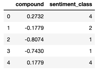
We make a seaborn countplot to show us the distribution of sentiment classes in the dataset:
import seaborn as sns# Distribution of sentiment_class
plt.figure(figsize = (10,5))
sns.set_palette('PuBuGn_d')
sns.countplot(data['sentiment_class'])
plt.title('Countplot of sentiment_class')
plt.xlabel('sentiment_class')
plt.ylabel('No. of classes')
plt.show()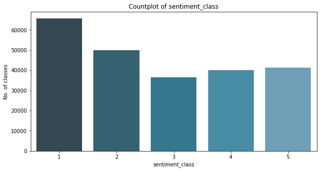
Let’s take a look at some of the tweets in each sentiment class:
- 10 random tweets that are classified with ‘negative sentiment’ — classes 1 and 2
# Display full text in Jupyter notebook:
pd.set_option('display.max_colwidth', -1)
# Look at some examples of negative, neutral and positive tweets# Filter 10 negative original tweets:
print("10 random negative original tweets and their sentiment classes:")
data[(data['sentiment_class'] == 1) | (data['sentiment_class'] == 2)].sample(n=10)[['text', 'sentiment_class']]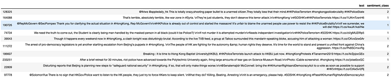
It is clear that the tweets are about denouncing alleged police violence, rallying for international support — especially from the United States — and reporting about police activities that are against the protesters.
2. 10 random tweets that are classified with ‘neutral sentiment’ — class 3
# Filter 10 neutral original tweets:
print("10 random neutral original tweets and their sentiment classes:")
data[(data['sentiment_class'] == 3)].sample(n=10)[['text', 'sentiment_class']]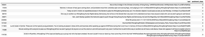
Most of these tweets, except for the last one with index 114113, are supposed to be neutral in stance. But given the context, it can be inferred that the tweets are about supporting the protesters and their cause.
3. 20 random tweets that are classified with ‘positive sentiment’ — classes 4 and 5
# Filter 20 positive original tweets:
print("20 random positive original tweets and their sentiment classes:")
data[(data['sentiment_class'] == 4) | (data['sentiment_class'] == 5)].sample(n=20)[['text', 'sentiment_class']]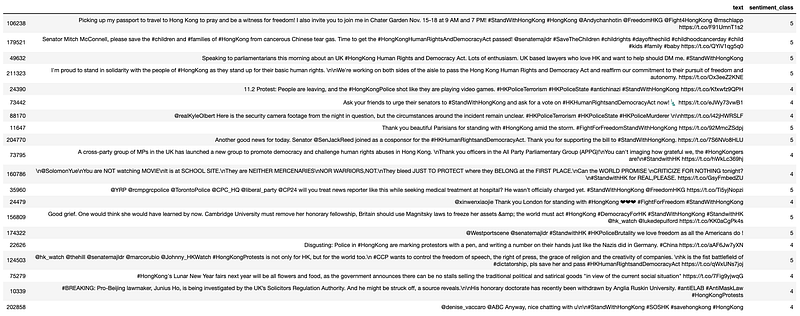
20 random tweets were picked out but almost, if not all, are actually negative in sentiments, which means they are against the Hong Kong government and/or police. A quick observation reveals that the tweets covered the topics: passing the Hong Kong Democracy and Human Rights Act in the United States; removing fellowships from Hong Kong politician(s); and generally supporting the Hong Kong protesters.
This supports the argument made earlier that a rule-based sentimental analysis of tweets using the Vader Lexicon library in this case is inaccurate in identifying REAL positive sentiments, leaving us with many false positives. It fails to examine and take the context of the tweets into account. Most of the ‘positive sentiment’ tweets contain more ‘positive’ words than ‘negative’ ones but they actually show support to the protesters and their cause, NOT to the Hong Kong government and/or China.
3. Popularity of Hashtags
Recall that the tweets were scraped using a pre-defined search term that contains a list of specific hashtags, pertaining to the protests. In addition, the tweets can also contain other hashtags that are not defined in the search term, as long as the tweet contains hashtag(s) that are/is defined by the search term.
In this section, we want to find out what are the most and least popular hashtags used by Twitter users in their tweets.
# the column data['hashtags'] returns a list of string(s) for each tweet. Build a list of all hashtags in the dataset.hashtag_list = []for i in range(0, len(data)):
# Obtain the current list of hashtags
curr_hashtag = data.iloc[i, :]['hashtags']
# Extract and append the hashtags to 'hashtag_list':
for j in range(0, len(curr_hashtag)):
hashtag_list.append(curr_hashtag[j])The total number of hashtags used can be determined by:
# No. of hashtags
print('No. of hashtags used in {} tweets is {}'.format(len(data), len(hashtag_list)))
No. of hashtags used in 233651 tweets is 287331
We build a simple dataframe for visualisation purposes:
df_hashtag = pd.DataFrame(
    {'hashtags': hashtag_list}
)print(df_hashtag.head())
print('Shape of df_hashtag is:', df_hashtag.shape)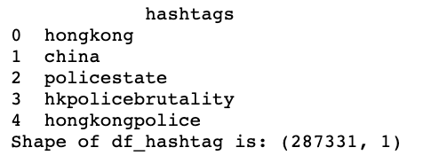
Basic Visualisation: All-time Top 15 Hashtags used
Let’s take a look at the top 15 hashtags used by users
# Define N to be the top number of hashtags
N = 15
top_hashtags = df_hashtag.groupby(['hashtags']).size().reset_index(name = 'counts').sort_values(by = 'counts', ascending = False).head(N)
print(top_hashtags)
# seaborn countplot on the top N hashtags
plt.figure(figsize=(30,8))
sns.set_palette('PuBuGn_d')
sns.barplot(x = 'hashtags', y = 'counts', data = top_hashtags)
plt.title('Barplot of Top ' + str(N) + ' Hashtags used')
plt.xlabel('Hashtags')
plt.ylabel('Frequency')
plt.show()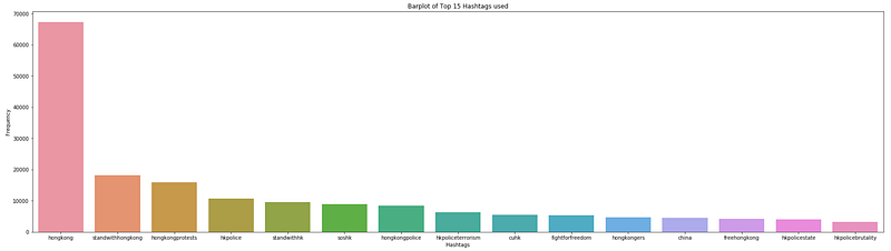
As expected, there are 14 out of 15 hashtags that contain the keywords ‘hong kong’ and ‘hk’ because users use them to identify their tweets with Hong Kong and the protests. The only hashtag that is different from the rest is #china.
There are 6 hashtags that explicitly show support to the protesters and decry about the Hong Kong police’s actions and behaviours — these hashtags are: #fightforfreedom, #freehongkong, #fightforfreedom, #hkpoliceterrorism, #hkpolicestate, and #hkpolicebrutality.
Advanced Visualisation: Time-series of Top 10 Hashtags over the Last 7 Days (Not exactly a time series…)
We want to see the growth in usage of hashtags starting from 3rd November 2019 when the scraping of data started. Did one or few hashtags become more popular over time? Let’s find out:
from datetime import datetimeind_to_drop = []
date = []# First find out which 'tweetcreatedts' is not a string or in other weird formats
for i in range(0, len(data)):
ith_date_str = data.iloc[i,:]['tweetcreatedts']
ith_match = re.search(r'\d{4}-\d{2}-\d{2}', ith_date_str)
if ith_match == None:
ind_to_drop.append(i)
else:
continue# Drop these rows using ind_to_drop
data.drop(ind_to_drop, inplace = True)# Create a new list of datetime date objects from the tweets:
for i in range(0, len(data)):
ith_date_str = data.iloc[i, :]['tweetcreatedts']
ith_match = re.search(r'\d{4}-\d{2}-\d{2}', ith_date_str)
ith_date = datetime.strptime(ith_match.group(), '%Y-%m-%d').date()
date.append(ith_date)
# Size of list 'date'
print('Len of date list: ', len(date))Len of date list: 233648
# Append 'date' to dataframe 'data' as 'dt_date' aka 'datetime_date'
data['dt_date'] = date
# Check to see that we have the correct list of dates from the dataset
data['dt_date'].value_counts()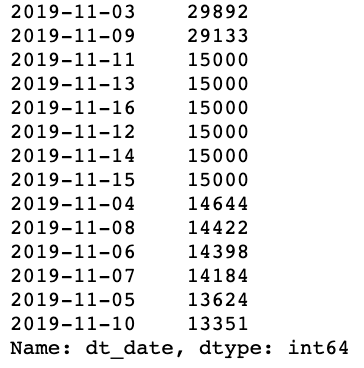
# Create a new dataframe first
timeseries_hashtags = pd.DataFrame(columns = ['hashtags', 'count', 'date', 'dayofnov'])
# Obtain a set of unique dates in 'date' list:
unique_date = np.unique(date)We define a function that allows you to choose the top N hashtags to show, and also data from the last T days, instead of everyday since 3rd Nov 2019 (although you can, it would clutter the plot)
def visualize_top_hashtags(main_df, timeseries_df, N, T, unique_dates):
    # main_df - main dataframe 'data'
    # timeseries_df - a new and empty dataframe to store the top hashtags
    # N - number of top hashtags to consider
    # T - number of days to consider
    # unique_dates - list of unique dates available in the table

    # Returns:
    # timeseries_df

    # Start counter to keep track of number of days already considered
    counter = 1
# Starting from the latest date in the list
for ith_date in reversed(unique_dates):
# Check if counter exceeds the number of days required, T:
if counter <= T:
# Filter tweets created on this date:
ith_date_df = main_df[main_df['dt_date'] == ith_date]# From this particular df, build a list of all possible hashtags:
ith_hashtag_list = []for i in range(0, len(ith_date_df)):
# Obtain the current list of hashtags:
curr_hashtag = ith_date_df.iloc[i,:]['hashtags']# Extract and append the hashtags to 'hashtag_list':
for j in range(0, len(curr_hashtag)):
ith_hashtag_list.append(curr_hashtag[j])# Convert the list into a simple DataFrame
ith_df_hashtag = pd.DataFrame({
'hashtags': ith_hashtag_list
})# Obtain top N hashtags:
ith_top_hashtags = ith_df_hashtag.groupby(['hashtags']).size().reset_index(name = 'count').sort_values(by = 'count', ascending = False).head(N)# Add date as a column
ith_top_hashtags['date'] = ith_date
ith_top_hashtags['dayofnov'] = ith_date.day# Finally, concat this dataframe to timeseries_hashtags
timeseries_df = pd.concat([timeseries_df, ith_top_hashtags], axis = 0)# Increase counter by 1
counter += 1
else: # break the for loop
break
print('The newly created timeseries_hashtag of size {} is: '.format(timeseries_df.shape))
timeseries_df.reset_index(inplace = True, drop = True)
# Visualization
plt.figure(figsize=(28,12))
ax = sns.barplot(x = 'hashtags',
y = 'count',
data = timeseries_df,
hue = 'dayofnov')# plt.xticks(np.arange(3, 6, step=1))
# Moving legend box outside of the plot
plt.legend(bbox_to_anchor=(1.05, 1), loc=2, borderaxespad=0.)
# for legend text
plt.setp(ax.get_legend().get_texts(), fontsize='22')
# for legend title
plt.setp(ax.get_legend().get_title(), fontsize='32')
plt.xlabel('Top Hashtags')
plt.ylabel('Count of Hashtags')
plt.title('Top ' + str(N) + ' Hashtags per day')
sns.despine(left=True, bottom=True)
plt.xticks(rotation = 45)
plt.show()
return timeseries_dfWe can finally make the plot:
timeseries_hashtags = visualize_top_hashtags(main_df = data,
                       timeseries_df = timeseries_hashtags,
                       N = 10,
                       T = 7,
                       unique_dates = unique_date)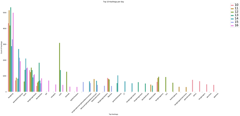
I figured that it would be easier to view the trend for each hashtag with a bar plot than with a scatter plot even though it would show the time-series, because it is harder to relate each point to the legend when there are so many colours and categories (hashtags).
A plot of top 10 hashtags per day for the past 7 days since 16 Nov 2019 show the commonly used hashtags for the movement — #hongkong, #hongkongprotests, #hongkongpolice, #standwithhongkong, and #hkpolice.
Other than the usual hashtags, the visualisation function can reveal unique and major events/incidents because users use these hashtags in their tweets when they talk about it.
Throughout the period, we see sudden appearance of hashtags such as #blizzcon2019 (not shown because of different parameters N and T), #周梓樂 (represented by squares in above graph), #japanese, #antielab, #pla, and #hkhumanrightsanddemocracyact.
These hashtags are tied to significant milestones:
- #blizzcon2019/blizzcon19 — https://www.scmp.com/tech/apps-social/article/3035987/will-blizzcon-become-latest-battleground-hong-kong-protests
- #周梓樂 — https://www.bbc.com/news/world-asia-china-50343584
- #hkust (related to #周梓樂) — https://www.hongkongfp.com/2019/11/08/hong-kong-students-death-prompts-fresh-anger-protests/
- #japanese (A japanese was mistaken to be a mainland chinese and hence, was attacked by the protesters) — https://www3.nhk.or.jp/nhkworld/en/news/20191112_36/#:~:targetText=Hong%20Kong%20media%20reported%20on,take%20pictures%20of%20protest%20activities.
- #antielab (protesters boycotting the elections because Joshua Wong was banned from it) — https://www.scmp.com/news/hong-kong/politics/article/3035285/democracy-activist-joshua-wong-banned-running-hong-kong
- #pla (China’s People’s Liberation Army (PLA) troops stationed in Hong Kong helped to clean and clear streets that were blocked and damaged by protesters) — https://www.channelnewsasia.com/news/asia/china-s-pla-soldiers-help-clean-up-hong-kong-streets-but-12099910
It is expected that major incidents will continue to trigger new hashtags in future, in addition to the usual ones.
4. Most Popular Tweets
In this section, we focus on what are the most popular tweets. There are 2 indicators that can help us achieve this — a tweet’s retweet count and favourite count. Unfortunately, we could only extract the retweet count because there was some trouble in retrieving the favourite count from the mess of dictionaries in the .json format (Please feel free to leave a comment if you know how to do it!).
We will do the following:
- Top N tweets of all time
- Top N tweets for particular day
- Top N tweets for the past T days
Top 10 Tweets of All Time
# Convert the data type of the column to all int using pd.to_numeric()print('Current data type of "retweetcount" is:',data['retweetcount'].dtypes)data['retweetcount'] = pd.to_numeric(arg = data['retweetcount'])print('Current data type of "retweetcount" is:',data['retweetcount'].dtypes)Current data type of “retweetcount” is: object Current data type of “retweetcount” is: int64
We define a function to pull out the top 10 tweets:
def alltime_top_tweets(df, N):
    # Arguments:
    # df - dataframe
    # N - top N tweets based on retweetcount

    # Sort according to 'retweetcount'
    top_tweets_df = df.sort_values(by = ['retweetcount'], ascending = False)
    # Drop also duplicates from the list, keep only the copy with higher retweetcount
    top_tweets_df.drop_duplicates(subset = 'text', keep = 'first', inplace = True)
    # Keep only N rows
    top_tweets_df = top_tweets_df.head(N)

    # Print out only important details
    # username, tweetcreatedts, retweetcount, original text 'text'
return top_tweets_df[['username', 'tweetcreatedts', 'retweetcount', 'text']]print('All-time top 10 tweets:')
print('\n')
alltime_top_tweets(data, 10)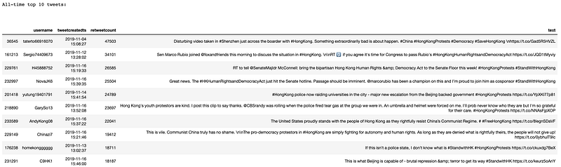
Top 10 Tweets for Any Particular Day
We can also create another function to pull out top N tweets for a specified day:
def specified_toptweets(df, spec_date, N):
    # Arguments
    # df - dataframe
    # N - top N tweets
    # date - enter particular date in str format i.e. '2019-11-02'

    # Specific date
    spec_date = datetime.strptime(spec_date, '%Y-%m-%d').date()

    # Filter df by date first
    date_df = df[df['dt_date'] == spec_date ]

    # Sort according to 'retweetcount'
    top_tweets_date_df = date_df.sort_values(by = ['retweetcount'], ascending = False)
    # Drop also duplicates from the list, keep only the copy with higher retweetcount
    top_tweets_date_df.drop_duplicates(subset = 'text', keep = 'first', inplace = True)
    # Keep only N rows
    top_tweets_date_df = top_tweets_date_df.head(N)

    print('Top ' + str(N) + ' tweets for date ' + str(spec_date) + ' are:')
    # Print out only important details
    # username, tweetcreatedts, retweetcount, original text 'text'
    return top_tweets_date_df[['username', 'tweetcreatedts', 'retweetcount', 'text']]
Let’s try 5th Nov 2019:
specified_toptweets(data, '2019-11-05', 10)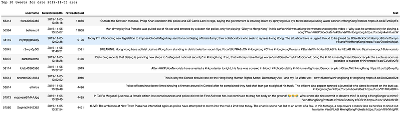
Top 2 Tweets for The Past 5 Days
Okay finally, we can also extract the top N tweets for the last T days with the following function:
def past_toptweets(df, T, N, unique_date):
    # Arguments:
    # df - dataframe 'data'
    # T - last T days
    # N - top N tweets
    # List of all unique dates in dataset

    # Create a df to store top tweets for all T dates, in case there is a need to manipulate this df
    past_toptweets_df = pd.DataFrame(columns = ['username', 'tweetcreatedts', 'retweetcount', 'text'])
    print(past_toptweets_df)

    # Filter data according to last T dates first:
    # Do a check that T must not be greater than the no. of elements in unique_date
    if T <= len(unique_date):
        unique_date = unique_date[-T:] # a list
    else:
        raise Exception('T must be smaller than or equal to the number of dates in the dataset!')

    # Print out top N for each unique_date one after another, starting from the latest:
    for ith_date in reversed(unique_date):
        # Filter tweets created on this date:
        ith_date_df = df[df['dt_date'] == ith_date]

        # Sort according to 'retweetcount'
        top_tweets_date_df = ith_date_df.sort_values(by = ['retweetcount'], ascending = False)
        # Drop also duplicates from the list, keep only the copy with higher retweetcount
        top_tweets_date_df.drop_duplicates(subset = 'text', keep = 'first', inplace = True)
        # Keep only N rows
        top_tweets_date_df = top_tweets_date_df.head(N)
        # Keep only essential columns
        top_tweets_date_df = top_tweets_date_df[['username', 'tweetcreatedts', 'retweetcount', 'text']]

        # Append top_tweets_date_df to past_toptweets_df
        past_toptweets_df = pd.concat([past_toptweets_df, top_tweets_date_df], axis = 0)

        # Print out the top tweets for this ith_date
        print('Top ' + str(N) + ' tweets for date ' + str(ith_date) + ' are:')
        # print only essential columns:
        print(top_tweets_date_df)
        print('\n')

return past_toptweets_dfpast_toptweets(data, T = 5, N = 2, unique_date = unique_date)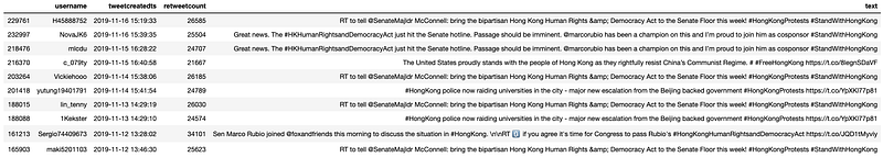
One flaw of the function ‘past_toptweets’ is that it can return tweets that are identical. For instance, a popular tweet on day 1 can be retweeted again on subsequent days by other users. This function can then pick up such tweets because no logic is implemented yet to consider only tweets that have not been chosen from earlier dates.
5. Behaviour of Twitter Users
No. of Tweets Daily
Let’s check out the trend in the number of tweets daily. We will build another dataframe that will be used to plot out the visualisation.
top_user_df = pd.DataFrame(columns = ['username', 'noTweets', 'noFollowers', 'dt_date'])# Convert datatype of 'totaltweets' to numeric
pd.to_numeric(data['totaltweets'])for ith_date in unique_date:
print('Current loop: ', ith_date)
temp = data[data['dt_date'] == ith_date]
# pd.DataFrame - count number of tweets tweeted in that day - noTweets
temp_noTweets = temp.groupby(['username']).size().reset_index(name = 'noTweets').sort_values(by = 'username', ascending = False)
# pd.Series - count max followers - might fluctuate during the day
temp_noFollowing = temp.groupby(['username'])['followers'].max().reset_index(name = 'noFollowers').sort_values(by = 'username', ascending = False)['noFollowers']
# *** NOT WORKING
# pd.Series - count max totaltweets - might fluctuate during the day. Note this is historical total number of tweets ever since the user is created.
# temp_noTotaltweets = temp.groupby(['username'])['totaltweets'].max().reset_index(name = 'noTotaltweets').sort_values(by = 'username', ascending = False)['noTotaltweets']
# Concat series to temp_noTweets, which will be the main df
final = pd.concat([temp_noTweets, temp_noFollowing], axis = 1) # add as columns
final['dt_date'] = ith_date
print(final)
# Append 'final' dataframe to top_user_df
top_user_df = pd.concat([top_user_df, final])Plotting the visualisation:
# hue = retweetcount and followers, totaltweets
f, axes = plt.subplots(3, 1, figsize = (22,22))
sns.set_palette('PuBuGn_d')
sns.stripplot(x = 'dt_date', y = 'noTweets', data = top_user_df, jitter = True, ax = axes[0], size = 6, alpha = 0.3)
sns.boxplot(y = 'dt_date', x = 'noTweets', data = top_user_df, orient = 'h', showfliers=False, ax = axes[1])
sns.boxplot(y = 'dt_date', x = 'noTweets', data = top_user_df, orient = 'h', showfliers=True, fliersize = 2.0, ax = axes[2])
# Axes and titles for each subplot
axes[0].set_xlabel('Date')
axes[0].set_ylabel('No. of Tweets')
axes[0].set_title('No. of Tweets Daily')axes[1].set_xlabel('No. of Tweets')
axes[1].set_ylabel('Date')
axes[1].set_title('No. of Tweets Daily')axes[2].set_xlabel('Date')
axes[2].set_ylabel('No. of Tweets')
axes[2].set_title('No. of Tweets Daily')plt.show()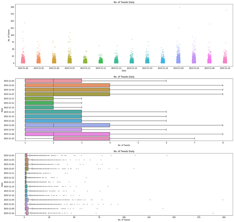
From the Seaborn box plots and strip plot, we see that most of the users in the dataset do not tweet a lot in a day. From the strip plot, we might not be able to discern the outliers in the dataset, and might think that most of the users tweeted in the range of 1 to 30 plus tweets daily.
However, the box plots tell us a different story. The first box plot in the middle of the visualisation reveals that most users tweeted roughly between 1 to 8 tweets. On the other hand, there are many outliers shown in the second box plot, at the bottom of the visualisation. These users tweeted a lot, ranging from 10 onwards. There were at least 7 users who have tweeted at least more than 100 tweets per day in the timeframe considered.
Top 5 Users with the Most Number of Tweets Daily
Let’s zoom in further by finding out who are top users exactly.
# To change the number of users, adjust the value in head()
# top_user_df.set_index(['dt_date', 'username']).sort_values(by = ['dt_date','noTweets'], ascending = False)
user_most_tweets_df = top_user_df.sort_values(by = ['dt_date', 'noTweets'], ascending = False, axis = 0).groupby('dt_date').head(5)
# Extract 'days' out of dt_date so we can plot a scatterplot
# Will return an int:
user_most_tweets_df['dayofNov'] = user_most_tweets_df['dt_date'].apply(lambda x: x.day)
user_most_tweets_df['noTweets'] = user_most_tweets_df['noTweets'].astype(int)# Plot 2 subplots
# 1st subplot - show who are the users who tweeted the most
# 2nd subplot - trend in number of tweets
f, axes = plt.subplots(2, 1, figsize = (20,20))
f = sns.scatterplot(x = 'dayofNov', y = 'noTweets', hue = 'username', data = user_most_tweets_df, size = 'noFollowers', sizes = (250, 1250), alpha = 0.75, ax = axes[0])
sns.lineplot(x = 'dayofNov', y = 'noTweets', data = user_most_tweets_df, markers = True)# Axes and titles for each subplot
# First subplot
axes[0].set_xlabel('Day in Nov')
axes[0].set_ylabel('No. of Tweets')
axes[0].set_title('Most no. of tweets daily')# Legends for first subplot
box = f.get_position()
f.set_position([box.x0, box.y0, box.width * 1.0, box.height]) # resize position# Put a legend to the right side
f.legend(loc='center right', bbox_to_anchor=(1.5, 0.5), ncol=4)# Second subplot
axes[1].set_xlabel('Date')
axes[1].set_ylabel('No. of Tweets')
axes[1].set_title('Trend of no. of tweets by top users')plt.show()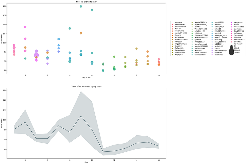
6. Demographics of Twitter Users
Location of Twitter Users
location = data['location']
print('No. of distinct locations listed by twitter users is:', len(location.value_counts()))
unique_locations = location.value_counts()
# Remove n.a.
unique_locations = pd.DataFrame({'locations': unique_locations.index,
'count': unique_locations.values})
unique_locations.drop(0, inplace = True)# See top few locations
unique_locations.sort_values(by = 'count', ascending = False).head(10)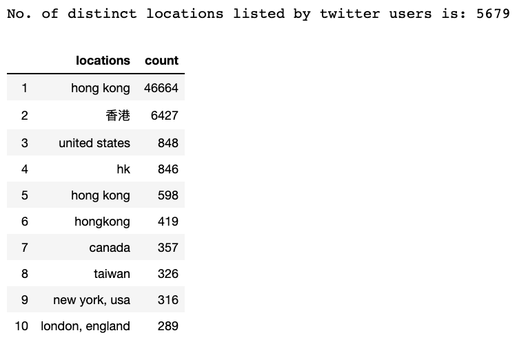
Expected to see that many of these users claim to be residing in Hong Kong since these users should be closer to the ground. Thus, they could spread news quickly from what they see in person.
We will discount ‘HongKong’ from the visualisation and focus on the distribution of the remaining locations:
# To remove 香港
hk_chinese_word = unique_locations.iloc[1,0]
# Obtain the row index of locations that contain hong kong:
ind_1 = unique_locations[unique_locations['locations'] == 'hong kong'].index.values[0]
ind_2 = unique_locations[unique_locations['locations'] == 'hk'].index.values[0]
ind_3 = unique_locations[unique_locations['locations'] == 'hong kong '].index.values[0]
ind_4 = unique_locations[unique_locations['locations'] == 'hongkong'].index.values[0]
ind_5 = unique_locations[unique_locations['locations'] == hk_chinese_word].index.values[0]
ind_6 = unique_locations[unique_locations['locations'] == 'kowloon city district'].index.values[0]list_ind = [ind_1,ind_2,ind_3,ind_4,ind_5, ind_6]# Drop these rows from unique_locations
unique_loc_temp = unique_locations.drop(list_ind)# Focus on top 20 locations first
# Convert any possible str to int/numeric first
count = pd.to_numeric(unique_loc_temp['count'])
unique_loc_temp['count'] = count
unique_loc_temp = unique_loc_temp.head(20)# Plot a bar plot
plt.figure(figsize=(16,13))
sns.set_palette('PuBuGn_d')
sns.barplot(x = 'count', y = 'locations', orient = 'h',data = unique_loc_temp)
plt.xlabel('Count')
plt.ylabel('Locations')
plt.title('Top 20 Locations')
plt.show()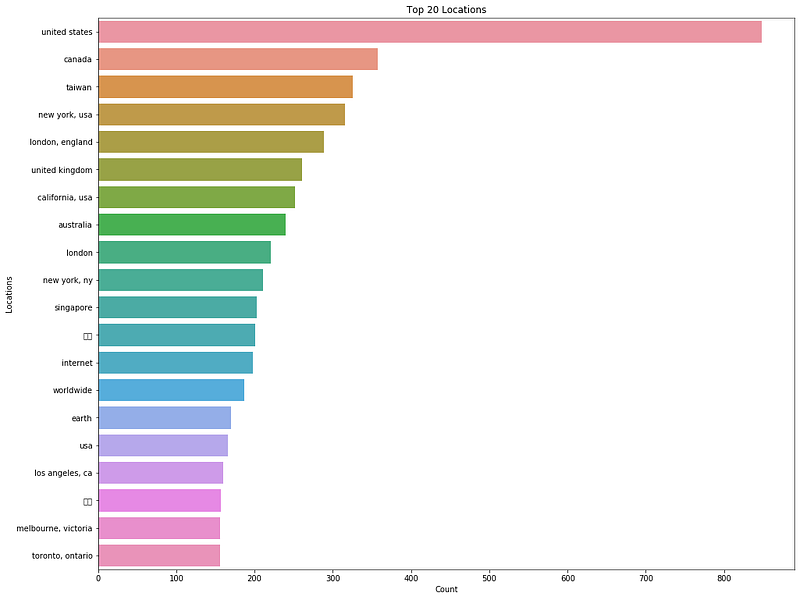
A quick count of the top 20 locations, without hong kong, shows that majority of these locations come from western countries. We see the expected ones such as the United States, Canada, UK and Australia, where some people and politicians are also watching over the protest movement and speaking out against the ruling government and police.
Top 30 Users with Most Followers
# Reuse code from top_user_df
# Sort according to noFollowers
top_user_df = top_user_df.sort_values(by = 'noFol lowers', ascending = False)
user_most_followers = top_user_df.groupby('username')['noFollowers', 'dt_date'].max().sort_values(by = 'noFollowers', ascending = False)
user_most_followers['username'] = user_most_followers.index
user_most_followers.reset_index(inplace = True, drop = True)
# plot chart
plt.figure(figsize = (25, 8))
sns.set_palette('PuBuGn_d')
sns.barplot(x = 'noFollowers', y = 'username', orient = 'h', data = user_most_followers.head(30))
plt.xlabel('No. of Followers')
plt.ylabel('Usernames')
plt.title('Top Twitter Accounts')
plt.show()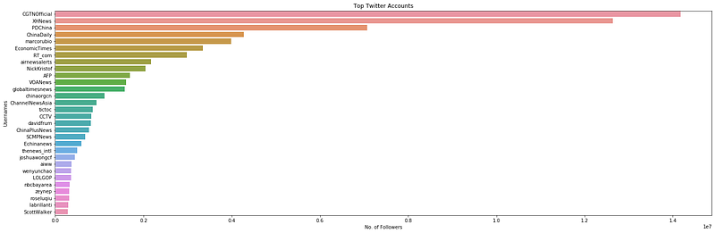
In the list of top 30 accounts, majority of them are accounts that belong to news agencies or media outlets such as AFP, CGTNOfficial, EconomicTimes, and ChannelNewsAsia. The rest belongs to individuals who are journalists and writers etc. Joshua Wong’s account is the only one in the list that can be identified as part of the protests.
Activities of Top Accounts
user_most_followers_daily = top_user_df.sort_values(by = ['dt_date', 'noFollowers'], ascending = False, axis = 0).groupby('dt_date').head(5)
print(user_most_followers_daily)
# Extract 'days' out of dt_date so we can plot a scatterplot
# Will return an int:
user_most_followers_daily['dayofNov'] = user_most_followers_daily['dt_date'].apply(lambda x: x.day)
user_most_followers_daily['noFollowers'] =
user_most_followers_daily['noFollowers'].astype(int)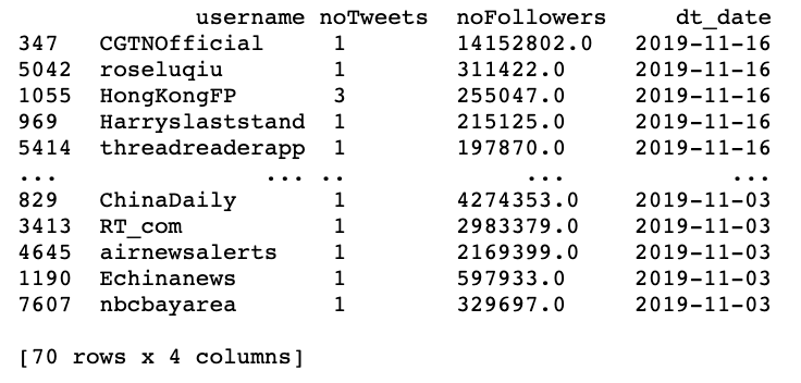
f, axes = plt.subplots(1, 1, figsize = (15,10))
f = sns.scatterplot(x = 'dayofNov', y = 'noTweets', hue = 'username',data = user_most_followers_daily, size = 'noFollowers', sizes=(50, 1000))
# Axes and titles for each subplot
# First subplot
axes.set_xlabel('Day in Nov')
axes.set_ylabel('No. of Tweets')
axes.set_title('Daily activity of users with most number of followers')# Legends for first subplot
box = f.get_position()
f.set_position([box.x0, box.y0, box.width * 1, box.height]) # resize position# Put a legend to the right side
f.legend(loc='center right', bbox_to_anchor=(1.5, 0.5), ncol=3)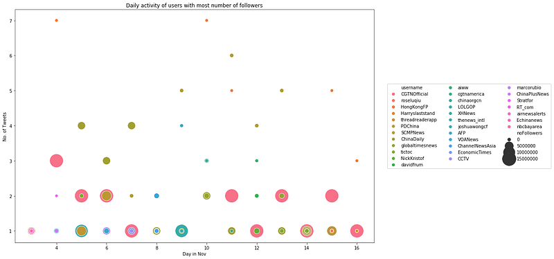
Although these top accounts have a lot of followers, the number of tweets they post per day, on average, is fewer than 10. This kind of activity pales in comparison as compared to that of the top 5 users with most number of tweets daily under the section ‘Top 5 Users with the Most Number of Tweets Daily’.
7. Most Mentioned Usernames
Can we uncover more popular figures in the protest movements from these tweets? Twitter users might be tagging these people to inform them of events that are happening on the ground. Their backgrounds can range from lawyers, lawmakers, politicians, reporters to even protest leaders.
def find_users(df):
    # df: dataframe to look at
    # returns a list of usernames

    # Create empty list
    list_users = []

    for i in range(0, len(df)):
        users_ith_text = re.findall('@[^\s]+', df.iloc[i,:]['text'])
        # returns a list
        # append to list_users by going through a for-loop:
        for j in range(0, len(users_ith_text)):
            list_users.append(users_ith_text[j])

    return list_users
# Apply on dataframe data['text']
list_users = find_users(data)mentioned_users_df = pd.DataFrame({
'mentioned_users': list_users
})mentionedusers = mentioned_users_df.groupby('mentioned_users').size().reset_index(name = 'totalcount').sort_values(by = 'totalcount', ascending = False)
mentionedusers.head()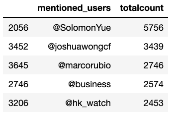
plt.figure(figsize=(30,8))
sns.set_palette('PuBuGn_d')
sns.barplot(x = 'mentioned_users', y = 'totalcount', data = mentionedusers.head(15))
plt.xlabel('Mentioned users in tweets')
plt.ylabel('Number of times')
plt.title('Top users and how many times they were mentioned in tweets')
plt.show()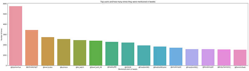
Most of the 15 most mentioned users, if not all, are directly related to Hong Kong and the protest movements. A quick google search on each of these users returns queries that show that they are either supportive of the protesters and protests and/or against the Hong Kong Administration and the police force. In summary:
- @SolomonYue — a Chinese American politician related to the Hong Kong Human Rights and Democracy Act passed in the U.S
- @joshuawongcf — a local protest leader who was planning to take part in the elections but was banned.
- @GOVUK — threatens to sanction hong kong officials over their handling of the protest
- @HawleyMO — a U.S politician
- @HeatherWheeler — Minister for Asia and the Pacific who sent a letter to Hong Kong government officials on the proposed sanctions.
Conclusion on EDA
All in all, more than 200k tweets regarding the Hong Kong Protest Movement 2019 over a period of 14 days starting from 3rd Nov 2019 till 16th Nov 2019 were scraped. The main steps required are setting up of Twitter API calls; cleaning and processing the tweets; and creating Seaborn visualisations. The data analysis/visualisation of this project focused on several themes:
- Most Popular Words with a Word Cloud
- Sentiment Analysis with Vader-Lexicon from NLTK
- Popularity of Hashtags
- Most Popular Tweets
- Activity of Twitter Users
- Demographic of Twitter Users
- Most Mentioned Usernames
Usefulness of Hashtags
NOTABLY, it is possible to identify significant milestones in the protests by monitoring the daily popularity and trend of the hashtags used by users. In theory, this means that one could simply monitor the hashtags and go without reading the news or scrolling through social media to keep updated with the protests movement.
Usefulness of Popular Tweets
THE most popular tweets can also help to reveal ongoing sentiments of the general twitter users pertaining to the movement. We can understand it as follows. When a tweet about a certain event or content gets retweeted by many people, it could mean that these people resonate with the message and want to share it to as many people as possible. As an example, the Hong Kong Human Rights and Democracy Act was such a hot topic. The most popular tweets can also provide further details and granularity as to what are the main topics/events for a day. In the evidence shown above in the section entitled ‘Most Popular Tweets’, we saw that these tweets often involve cases about police brutality and alleged inappropriate use of force.
Personal Observation
AFTER completing this project, it has strengthened my belief that the overall sentiment towards a topic/idea might be dependent on the social media platform i.e. Twitter, Facebook, Weibo etc.
So far we have seen that the overall sentiment of the Hong Kong protest movement from these Twitter tweets are overwhelming negative towards the Hong Kong Government and the police force, but positive and supportive towards the protesters. Likewise, we might get an opposite reaction on platforms like Weibo and other Chinese media sites that show support and praise for the Hong Kong government and police.
Nevertheless, it is also possible that I am wrong and there was a flaw in the collection of tweets because of the hashtags used in the search term. Hashtags used in our search were explicitly about the negative aspects of the police such as #hkpolicebrutality. People who used it used it obviously to denounce these alleged brutality. In retrospection, it would be fairer to consider hashtags such as #supporthongkongpolice #supporthkgovt #supporthkpolice etc. I will leave this to the reader to explore this element.
Shortcomings of Ruled-Based Sentiment Analysis
THE rudimentary sentiment analysis that we did above using the Vader Library from NLTLK revealed plenty of false positives — upon closer inspection of these random tweets that were rated to be positive towards the government and police, they actually turned out to be either negative towards them or supportive towards the protesters’ cause. Hence, we need to turn to deep learning techniques that would give us better and reliable results.
It is not within the scope and aim of this project to cover the deep learning work. More work needs to be done in classifying a small dataset of tweets, so that it could be used for transfer learning with pre-trained models.
However, based on the tweets we have on hand, there has been an overwhelming support for the protesters and their cause, but public outcry over police brutality and misbehaviours. Any attempts at classifying the tweets into positive or negative sentiments might end up with a highly skewed distribution of negative sentiments towards the Hong Kong Government and Police Force. Hence, it might not be worthwhile to proceed with predicting the sentiments with deep learning. In my opinion, the sentiment of related Twitter tweets is largely negative.
Cleaning up and Preprocessing the Tweets
From here onwards, readers who are keen in the flow of data cleaning for this project may continue to walk through the remainder sections of this article.

Import Libraries and Dataset
In a separate Jupyter Notebook:
# Generic ones
import numpy as np
import pandas as pd
import os
# Word processing libraries
import re
from nltk.corpus import wordnet
import string
from nltk import pos_tag
from nltk.corpus import stopwords
from nltk.tokenize import WhitespaceTokenizer
from nltk.stem import WordNetLemmatizer# Widen the size of each cell
from IPython.core.display import display, HTML
display(HTML("<style>.container { width:95% !important; }</style>"))Each round of tweet scraping results in a creation of a .csv file. Read each .csv file into a dataframe first:
# read .csv files into Pandas dataframes first
tweets_1st = pd.read_csv(os.getcwd() + '/data/raw' + '/20191103_131218_sahkprotests_tweets.csv', engine='python')
..
..
tweets_15th = pd.read_csv(os.getcwd() + '/data/raw' + '/20191116_121136_sahkprotests_tweets.csv', engine='python')
# Check the shape of each dataframe:
print('Size of 1st set is:', tweets_1st.shape)# You can also check out the summary statistics:
print(tweets_1st.info())Concatenate all dataframes into a single dataframe:
# Concat the two dataset together:
data = pd.concat([tweets_1st, tweets_2nd, tweets_3rd, tweets_4th, tweets_5th, tweets_6th, tweets_7th, tweets_8th, tweets_9th, tweets_10th, tweets_11th, tweets_12th, tweets_13th, tweets_14th, tweets_15th], axis = 0)print('Size of concatenated dataset is:', data.shape)# Reset_index
data.reset_index(inplace = True, drop = True)
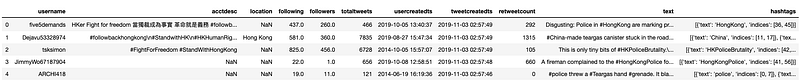
data.head()
print(data.info())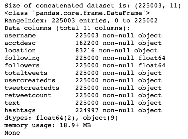
A snippet of what you will see in the dataframe:
Checking for Duplicated Entries and Removing Them
Since we are performing the scraping close to each other, it is possible to scrape the same tweets as long as they fall within the search window of 7 days from the search_date. We remove these duplicated rows from our dataset.
# Let's drop duplicated rows:
print('Initial size of dataset before dropping duplicated rows:', data.shape)
data.drop_duplicates(keep = False, inplace = True)print('Current size of dataset after dropping duplicated rows, if any, is:', data.shape)Initial size of dataset before dropping duplicated rows: (225003, 11) Current size of dataset after dropping duplicated rows, if any, is: (218652, 11)
Remove Non-English Words/Tokens
Since it might be possible to remove non-English words that are used in daily English conversations such as names etc, it might be better to filter by the Chinese language.
# Remove empty tweets
data.dropna(subset = ['text'], inplace = True)
# The unicode accounts for Chinese characters and punctuations.
def strip_chinese_words(string):
# list of english words
en_list = re.findall(u'[^\u4E00-\u9FA5\u3000-\u303F]', str(string))
# Remove word from the list, if not english
for c in string:
if c not in en_list:
string = string.replace(c, '')
return string# Apply strip_chinese_words(...) on the column 'text'
data['text'] = data['text'].apply(lambda x: strip_chinese_words(x))
data.head()Extract Twitter Usernames Mentioned in Each Tweet
We want this useful information from each tweet because we can analyse who are the popular figures in the protest movement.
# Define function to sieve out @users in a tweet:
def mentioned_users(string):
    usernames = re.findall('@[^\s]+', string)
    return usernames
# Create a new column and apply the function on the column 'text'
data['mentioned_users'] = data['text'].apply(lambda x: mentioned_users(x))
data.head()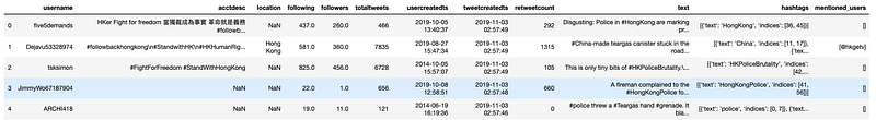
Main Text Cleaning and Preprocessing
With Chinese words and usernames removed and extracted from each text, we can now do the heavy lifting:
# Define Emoji_patterns
emoji_pattern = re.compile("["
         u"\U0001F600-\U0001F64F"  # emoticons
         u"\U0001F300-\U0001F5FF"  # symbols & pictographs
         u"\U0001F680-\U0001F6FF"  # transport & map symbols
         u"\U0001F1E0-\U0001F1FF"  # flags (iOS)
         u"\U00002702-\U000027B0"
         u"\U000024C2-\U0001F251"
         "]+", flags=re.UNICODE)
# Define the function to implement POS tagging:
def get_wordnet_pos(pos_tag):
if pos_tag.startswith('J'):
return wordnet.ADJ
elif pos_tag.startswith('V'):
return wordnet.VERB
elif pos_tag.startswith('N'):
return wordnet.NOUN
elif pos_tag.startswith('R'):
return wordnet.ADV
else:
return wordnet.NOUN# Define the main function to clean text in various ways:
def clean_text(text):
# Apply regex expressions first before converting string to list of tokens/words:
# 1. remove @usernames
text = re.sub('@[^\s]+', '', text)
# 2. remove URLs
text = re.sub('((www\.[^\s]+)|(https?://[^\s]+))', '', text)
# 3. remove hashtags entirely i.e. #hashtags
text = re.sub(r'#([^\s]+)', '', text)
# 4. remove emojis
text = emoji_pattern.sub(r'', text)
# 5. Convert text to lowercase
text = text.lower()
# 6. tokenise text and remove punctuation
text = [word.strip(string.punctuation) for word in text.split(" ")]
# 7. remove numbers
text = [word for word in text if not any(c.isdigit() for c in word)]
# 8. remove stop words
stop = stopwords.words('english')
text = [x for x in text if x not in stop]
# 9. remove empty tokens
text = [t for t in text if len(t) > 0]
# 10. pos tag text and lemmatize text
pos_tags = pos_tag(text)
text = [WordNetLemmatizer().lemmatize(t[0], get_wordnet_pos(t[1])) for t in pos_tags]
# 11. remove words with only one letter
text = [t for t in text if len(t) > 1]
# join all
text = " ".join(text)
return(text)# Apply function on the column 'text':
data['cleaned_text'] = data['text'].apply(lambda x: clean_text(x))
data.head()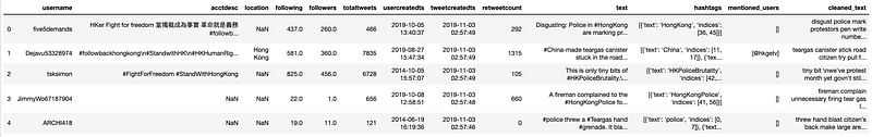
# Check out the shape again and reset_index
print(data.shape)
data.reset_index(inplace = True, drop = True)
# Check out data.tail() to validate index has been reset
data.tail()Process the Column ‘hashtags’
The data type of the column ‘hashtags’ is initially in string, so we need to convert it to a Python list.
# Import ast to convert a string representation of list to list
# The column 'hashtags' is affected
import ast
# Define a function to convert a string rep. of list to list
## Function should also handle NaN values after conversion
def strlist_to_list(text):
# Remove NaN
if pd.isnull(text) == True: # if true
text = ''
else:
text = ast.literal_eval(text)
return text# Apply strlist_to_list(...) to the column 'hashtags'
# Note that doing so will return a list of dictionaries, where there will be one dictionary for each hashtag in a single tweet.
data['hashtags'] = data['hashtags'].apply(lambda x: strlist_to_list(x))data.head()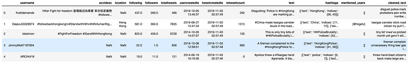
Since each ‘hashtag’ entry contains a list of dictionaries, we need to loop through the list to extract each hashtag:
# Define a function to perform this extraction:
def extract_hashtags(hashtag_list):
    # argument:
    # hashtag_list - a list of dictionary(ies), each containing a hashtag

    # Create a list to store the hashtags
    hashtags = []

    # Loop through the list:
    for i in range(0, len(hashtag_list)):
        # extract the hashtag value using the key - 'text'
        # For our purposes, we can ignore the indices, which tell us the position of the hashtags in the string of tweet
        # lowercase the text as well
        hashtags.append(hashtag_list[i]['text'].lower())

    return hashtags
# Apply function on the column - data['hashtags']
data['hashtags'] = data['hashtags'].apply(lambda x: extract_hashtags(x))# Check out the updated column 'hashtags'
print(data.head()['hashtags'])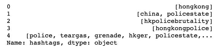
Process the Column ‘location’
# Replace NaN (empty) values with n.a to indicate that the user did not state his location
# Define a function to handle this:
def remove_nan(text):
    if pd.isnull(text) == True: # entry is NaN
        text = 'n.a'
    else:
        # lowercase text for possible easy handling
        text = text.lower()

    return text
# Apply function on column - data['location']
data['location'] = data['location'].apply(lambda x: remove_nan(x))# Check out the updated columns
print(data.head()['location'])# Let's take a quick look at the value_counts()
data['location'].value_counts()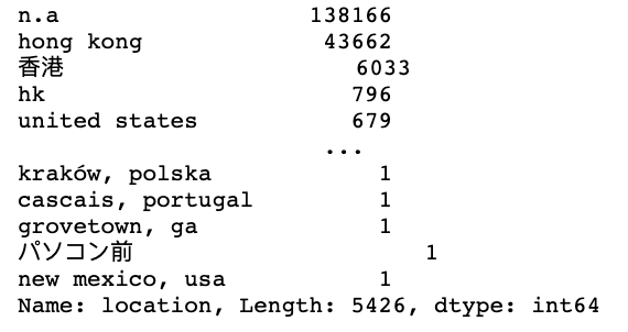
Unsurprisingly, most of the tweets are tweeted by users who are from/in Hong Kong. Since these are the locations of users of each tweet, it is still early to determine the actual demographics. We will deal with this later.
Process the Column ‘acctdesc’
We clean up this column — the account descriptions of twitter users — by removing NaN values and replacing them with string ‘n.a’.
# Apply the function already defined above: remove_nan(...)
# Apply function on column - data['acctdesc']
data['acctdesc'] = data['acctdesc'].apply(lambda x: remove_nan(x))
# Check out the updated columns
print(data.head()['acctdesc'])Feature Engineering — Rule-based Word Processing
So far, we have removed duplicated rows, extracted important information such as hashtags, mentioned users and users’ locations, and also cleaned up the tweets. In this section, we focus on rule-based word processing for our sentiment analysis. Exploratory data visualisation will be done later once we have all the ingredients.
Generate Sentiments from Tweets with NLTK Vader_Lexicon Library
We use the Vader_lexicon library from NLTK to generate sentiment for each tweet. Vader uses a lexicon of words to determine which words in the tweet are positive or negative. It will then return a set of 4 scores on the positivity, negativity, neutrality of the text, and also an overall score whether the text is positive or negative. We will define the following:
- Positivity — ‘pos’
- Negativity — ‘neg’
- Neutrality — ‘neu’
- Overall Score — ‘compound’
# Importing VADER from NLTK
from nltk.sentiment.vader import SentimentIntensityAnalyzer
# Create a sid object called SentimentIntensityAnalyzer()
sid = SentimentIntensityAnalyzer()# Apply polarity_score method of SentimentIntensityAnalyzer()
data['sentiment'] = data['cleaned_text'].apply(lambda x: sid.polarity_scores(x))# Keep only the compound scores under the column 'Sentiment'
data = pd.concat([data.drop(['sentiment'], axis = 1), data['sentiment'].apply(pd.Series)], axis = 1)Extract additional Features — no. of characters and no. of words in each tweet
# New column: number of characters in 'review'
data['numchars'] = data['cleaned_text'].apply(lambda x: len(x))
# New column: number of words in 'review'
data['numwords'] = data['cleaned_text'].apply(lambda x: len(x.split(" ")))# Check the new columns:
data.tail(2)
Word Embeddings — Training Doc2Vec using Gensim
Word embeddings involve the mapping of words in the text corpus to numerical vectors, where similar words sharing similar contexts will have similar vectors as well. It involves a shallow two-layer neural network that trains a matrix/tensor called the embedding matrix. By taking the matrix product of the embedding matrix and one-hot vector representation of each word in the corpus, we obtain the embedding vector.
We will use Gensim — an open-source Python library — to generate doc2vec.
Note: doc2vec should be used over word2vec to obtain the vector representation of a ‘document’, in this case, an entire tweet. Word2vec will only give us the vector representation of a word in a tweet.
# Import the Gensim package
from gensim.test.utils import common_texts
from gensim.models.doc2vec import Doc2Vec, TaggedDocument
documents = [TaggedDocument(doc, [i]) for i, doc in enumerate(data["cleaned_text"].apply(lambda x: x.split(" ")))]# Train a Doc2Vec model with our text data
model = Doc2Vec(documents, vector_size = 10, window = 2, min_count = 1, workers = 4)# Transform each document into a vector data
doc2vec_df = data["cleaned_text"].apply(lambda x: model.infer_vector(x.split(" "))).apply(pd.Series)
doc2vec_df.columns = ["doc2vec_vector_" + str(x) for x in doc2vec_df.columns]
data = pd.concat([data, doc2vec_df], axis = 1)# Check out the newly added columns:
data.tail(2)
Compute TD-IDF Columns
Next, we will compute the TD-IDF of the reviews using the sklearn library. TD-IDF stands for Term Frequency-Inverse Document Frequency, which is used to reflect how important a word is to a document in a collection or corpus. The TD-IDF value increases proportionally to the number of times a word appears in the document and is offset by the number of documents in the corpus that contain the word, which helps to adjust for the fact that some words appear more frequently in general.
- Term Frequency — the number of times a term occurs in a document.
- Inverse Document Frequency — an inverse document frequency factor that diminishes the weight of terms that occur very frequently in the document set and increases the weight of terms that occur rarely.
Since NLTK does not support TF-IDF, we will use the tfidfvectorizer function from the Python sklearn library.
from sklearn.feature_extraction.text import TfidfVectorizer# Call the function tfidfvectorizer
# min_df is the document frequency threshold for ignoring terms with a lower threshold.
# stop_words is the words to be removed from the corpus. We will check for stopwords again even though we had already performed it once previously.
tfidf = TfidfVectorizer(
max_features = 100,
min_df = 10,
stop_words = 'english'
)# Fit_transform our 'review' (the corpus) using the tfidf object from above
tfidf_result = tfidf.fit_transform(data['cleaned_text']).toarray()# Extract the frequencies and store them in a temporary dataframe
tfidf_df = pd.DataFrame(tfidf_result, columns = tfidf.get_feature_names())# Rename the column names and index
tfidf_df.columns = ["word_" + str(x) for x in tfidf_df.columns]
tfidf_df.index = data.index# Concatenate the two dataframes - 'dataset' and 'tfidf_df'
# Note: Axis = 1 -> add the 'tfidf_df' dataframe along the columns or add these columns as columns in 'dataset'.
data = pd.concat([data, tfidf_df], axis = 1)# Check out the new 'dataset' dataframe
data.tail(2)
Closing
I hope you have gained as much insights as I have. Feel free to leave a comment to share your thoughts or correct me on any technical aspects or my analysis of the data.
Thank you for your time in reading this lengthy article.