Simple lesson on investing

Analyse Stocks with Key Market Indicators (KMI) In 10 Minutes

Simple Python Codes to analyse Market Prices

Problem Statement

What do we look at when we look into stocks?

What are the basic tools to get started with stocks quickly?

How do we know when we should enter and exit the stocks market?

Given the ease of setting up trading accounts in the middle of pandemic, many have turned around to personal investing. And if you are reading this article, then congratulations, this will be your first step to learn.

If you want to trade, you would need to ask these questions to start:

1. What stocks to buy? (Value)
2. When to buy or sell the stocks? (Momentum)

I have covered the first question in Value Investing. So in this publication, I would focus on defining momentum in Key Market Indicators (KMI).

The objective for this publication is for you to understand one way of analyzing stocks momentum with KMI using quick and dirty Python Code. Just spend 10 minutes to read this article — or even better, contribute. Then you could get a quick glimpse to code your first financial analysis with KMI.

Over 3 years of investing, I have received 62% of Stocks Portfolio Returns. This method is simple and includes the peace of mind that often eludes risky investors.

Disclosure: This is a reflection from my personal investment results over value investing methodology over the past three years. This post is not meant to launch an agenda outside of personal sharing and reflections. If you are looking for a starting point to analyze stocks with data. Here are some guidelines from me.

With that, let’s jump into it!

Instructions

Colab Notebook

In this tutorial I provide a Google Colab (Colaboratory) Notebook to provide a data analysis repo for you to play around with it out yourself. It combines code, output, and descriptive text into one document — Further tutorial.

You can just click “Runtime > Run All” on Google Colab to run all the codes and generate the graphs. You can also change the file repository by defining a new Github link in link variable.

Finally, you can save all charts you created by uncommenting the following line. Define variable “title” to name the picture title.

plt.savefig(f’{title}.png’)

Import Data

I borrowed Raj Shah’s Google Stocks Price CSV data which is hosted publicly on Github. The code and the charts are presented below.

import pandas as pd
import requests
import numpy as np
import matplotlib.pyplot as plt
import datetime as dt

# Feel free to change the link to any you want or maybe web scrape the value.https://towardsdatascience.com/value-investing-dashboard-with-python-beautiful-soup-and-dash-python-43002

link = ‘https://raw.githubusercontent.com/raj-shah14/Predicting-Google-Stock-Prices/master/Google_Stock_Price_Train.csv'

r = requests.get(link, headers = {‘User-Agent’:’Mozilla/5.0 (Windows NT 10.0; Win64; x64) AppleWebKit/537.36 (KHTML, like Gecko) Chrome/91.0.4472.124 Safari/537.36'})

pandas_data = pd.read_csv(link)

print(pandas_data)

Data Cleaning

In most analysis of the key indicators, it is good to forwardfill and backfill the data to close the gap of missing dates in unclean stocks data. This is to prevent propagating null values in our analysis and use the nearest existing future dataset to cover the missing dates.

# Forward/backward fill the missing dates

def ffill_bfill(prices):
   prices_temp = prices.copy()
   prices_temp = prices_temp.fillna(method='ffill')
   prices_temp = prices_temp.fillna(method='bfill')
   return prices_temp

Simple Moving Average (SMA)

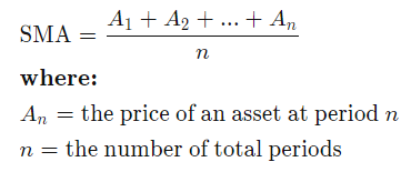
SMA is a tool that is commonly used by many analysts to predict security price changes. It averages the prices within a window to identify overall trends and cycles. This is calculated through the rolling mean of the stock’s normalized price. Each data point is averaged equally in each period of the rolling window.

Why does this work?

SMA aids in determining whether the asset price will keep increasing or will be reversed by looking at the mean average for each window. Short term averages respond relatively quickly to price changes in any given stock market while long term averages are slow to react to price changes.

Programmatically, we assign calculate the formula as the following:

Prices (normalized).rolling(window).mean()

With signals:
* Overbought signals: Price/SMA Ratio >1.05
* Oversold signals: Price/SMA Ratio< 0.95(stockscharts.com):

We can extract the SMA using the following codes

def get_sma (prices,window):
   prices_temp = prices.copy()
   sma = prices_temp.rolling(window=window).mean()
   sma.columns = [‘sma’]
   return sma

def get_psma(prices,sma):
   prices_temp = prices.copy()
   psma = prices_temp/sma
   return psma

price_df['sma'] = get_sma(price_df['Price'],10)
price_df['psma'] = get_psma(price_df['Price'],price_df['sma'])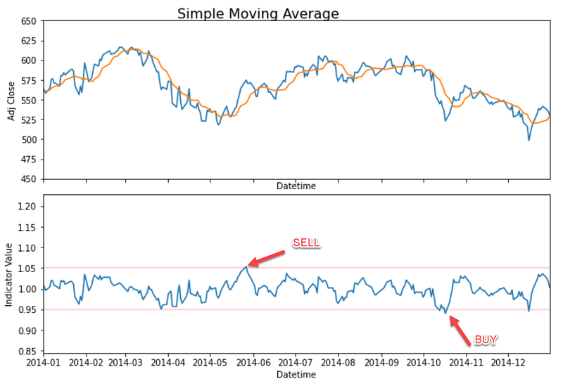

Bollinger Bands Percent (BB / BBP)

The Bollinger Bands are charted by drawing lines with 2 standard deviations gaps from the mean at any given time. These standard deviations are used with normalized prices similar to SMA.

Prices (normalized).rolling(window = 20).std()

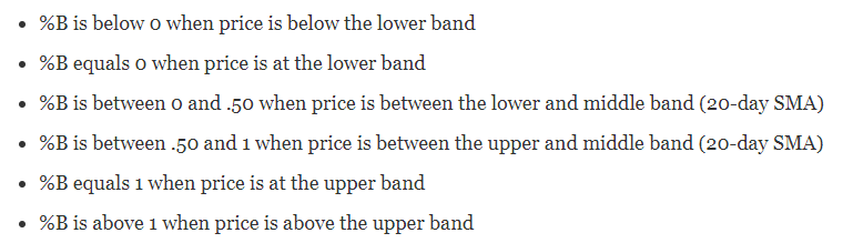
In this case, we are using the Bollinger Bands Percent (BBP) because the signal for buying and action is clearer. This quantifies security price in proportion to how near it is to the upper and lower BB. According to the stockscharts.com, these are the basic relationship levels:

With signals:
* BBP = (Price — Lower bands) / (Upper Bands — Lower Bands)
* Overbought scans → BBP >1
* Oversold scans → BBP <0

Why does this work?

BBP works because it signals overbought and oversold circumstances. This identifies the ideal situations where we want to look for correlation of short term situations with the medium term. Ideally when the medium trend is up, the short term is oversold, but when the medium trend is down, the short term is overbought.

It works by quantifying the price closer to its BB upper and lower which indicates strong overbought or strong oversold. By using this, we can still identify the trends with BB while quantifying its situation to trigger actions when the entry point is right.

def get_bollinger_bands(prices, window, sma):
   prices_temp = prices.copy()
   std = prices_temp.rolling(window=window, min_periods=window).std()
   std.columns=[‘sma’]
   bb = pd.DataFrame(index=prices.index,columns = [‘Lower’,’Upper’])
   bb[‘Upper’] = sma + std * 2
   bb[‘Lower’] = sma — std * 2
   bb[‘Price’] = prices_temp
   return bb

def get_bbp(bb):
   bbp = (bb[‘Price’] — bb[‘Lower’])/(bb[‘Upper’] — bb[‘Lower’])
   bbp_df = bbp.to_frame()
   bbp_df.columns=[‘bbp’]
   return bbp_df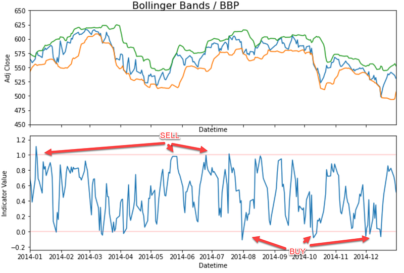

Relative Strength Index (RSI Momentum Indicator)

RSI is a momentum indicator to identify the price changes magnitude to signal overbought and oversold. RSI can be displayed as an oscillator with 0 to 100 readings and can be set with a standard 14 periods of days/weeks.

The formula includes calculating momentum through the stock price differences over a window period with the early price as the denominator.

RSI = 100–100/(1+Average gain/average loss)
Signals:
* Overbought signals = RSI > 70
* Oversold Signals = RSI <=0

Why does this work?

Momentum allows us to programmatically identify the oscillation signals. This means we can identify if the indicator fluctuates back and forth. Signals can arise when we look for divergences, oscillator swings, and centerline crosses.

Through these signals, traders could identify bullish and bearish momentum. This allows traders to take advantage of the market sentiment to predict rising or declining stocks prices until the opposite swing comes. This is a good match to compare with SMA and BBP Short which respond relatively quickly to price changes in the stocks market.

def get_rsi(prices, sd, periods= 14):
   prices_temp = prices.copy()
   prices_temp[‘up’] = 0
   prices_temp[‘down’] = 0
   prices_temp[‘rsi’] = 0
   for index,row in prices_temp.iterrows():
      current_datetime = index
      prev_day = current_datetime-dt.timedelta(days=1)
      try:
         if prev_day >= sd:
            prev_price = prices_temp.loc[prev_day,’Price’]
         if prev_price < row[‘Price’]:
            prices_temp.loc[index,’up’] = row[‘Price’] — prev_price
         elif prev_price > row[‘Price’]:
            prices_temp.loc[index,’down’] = prev_price — row[‘Price’]
      except:
         continue
      up_ewm = prices_temp[‘up’].ewm(span=periods).mean()
      down_ewm = prices_temp[‘down’].ewm(span=periods).mean()
      prices_temp[‘rsi’] = round(up_ewm/(up_ewm+down_ewm) * 100,0)
      added_date = sd + dt.timedelta(days=(periods-1))
      prices_temp.loc[:added_date,’rsi’] = np.nan
   return prices_temp[[‘rsi’]]

price_df['rsi'] = get_rsi(price_df,dt.datetime(2008,1,28))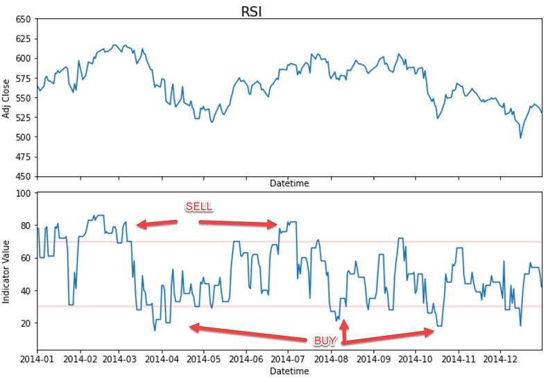

MACD

Similar to RSI, MACD also uses momentum indicators which plots relationships among two Moving Averages. The formula subtracts 26 periods from 12 periods of Exponential Moving Averages (EMA). Apart from the MACD formula, we also identify the signal line which is calculated within 9 days EMA. We will put BUY actions if MACD crosses above the signal line and SELL when MACD crosses below its signal line.

# From Investopedia
MACD = 12 Period EMA — 26 Period EMA 

Why does this work?

MACD suggests signal lines to identify buy or sell signals. Traders may use MACD to buy when the line crosses above the signal line and sell when the line crosses below the signal line. It identifies accelerations in data points to identify entry points and leverages the usage of Exponential Moving Average (EMA) used in tandem with RSI to paint a clearer picture of momentum in the market.

def get_macd(prices):
   exp_1 = prices.ewm(span=12,adjust=False).mean()
   exp_2 = prices.ewm(span=26,adjust=False).mean()
   macd_list = exp_1 — exp_2
   signal_macd_list = macd_list.ewm(span=9, adjust=False).mean()
   macd_df = pd.concat([macd_list,signal_macd_list],axis=1)
   macd_df.columns = [‘macd’,’signal’]
   return macd_df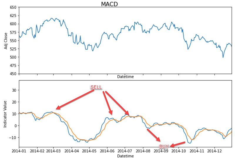

On Balance Volume (OBV)

OBV is a Volume based signal which uses volume flow to predict stocks price changes by using Volume data. The higher the OBV is, the higher the prices move. vice versa. This signals huge demands for certain stocks.

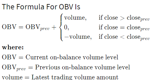
Signal:
* When the closing price today is higher, then current OBV = previous OBV + today’s volume.
* When closing price today is lower, then current OBV = previous OBV — today’s volume.
* When today’s closing price = yesterday’s closing price, current OBV = previous OBV

Why does this work?

OBV leverages on crowd sentiment which is helpful to predict bullish or bearish outcomes. It compares signals which identify volume histograms at the bottom of the price charts. This helps analysts track investors and the relationship among volume and price in a sequential timeline. Ideally, this can be paired up with other indicators such as (SMA, BBP, and RSI) to keep track of changes in prices and determine trends of stocks price movement.

def get_obv(prices,sd,volume):
   price_temp = prices.copy()
   volume_temp = volume.copy()
   price_temp.columns = [‘Price’]
   volume_temp.columns = [‘Volume’]
   price_temp[‘Volume’] = volume_temp[‘Volume’]
   price_temp[‘obv’] = 0
   for index, row in price_temp.iterrows():
      try:
         current_datetime = index
         prev_day = current_datetime-dt.timedelta(days=1)
         if prev_day >= sd:
            prev_price = price_temp.loc[prev_day,’Price’]
            prev_obv = price_temp.loc[prev_day,’obv’]
         if prev_price < row[‘Price’]:
            price_temp.loc[index,’obv’] = prev_obv + row[‘Volume’]
         elif prev_price > row[‘Price’]:
            price_temp.loc[index,’obv’] = prev_obv — row[‘Volume’]else:
            price_temp.loc[index,’obv’] = prev_obv
       except:
         continue
   return price_temp[[‘obv’]]

price_df['obv'] = get_obv(price_df[['Price']],dt.datetime(2008,1,28),volume_df)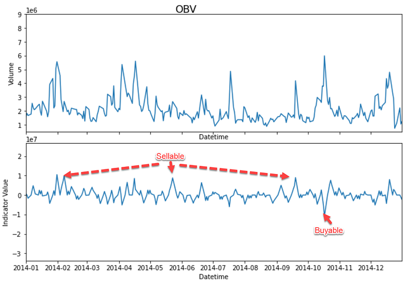

With that, I hope you can get started in looking these signals and purchase your stocks.

Happy Coding and Trying :)

About the Author

Vincent fights internet abuse with ML @ Google. Vincent uses advanced data analytics, machine learning, and software engineering to protect Chrome and Gmail users.

Apart from his stint at Google, Vincent is also Georgia Tech CS MSc Alumni, a triathlete, and a featured writer for Towards Data Science Medium to guide aspiring ML and data practitioners with 1M+ viewers globally.

Lastly, please reach out to Vincent via LinkedIn, Medium or Youtube Channel

Soli deo gloria

References

• Google Graph Mining and Learning
• Graph Neural Networks in TF and Keras with Spektral