
An Intuitive Explanation of Field Aware Factorization Machines
From LM to Poly2 to MF to FM to FFM
In the context of recommender systems, Field Aware Factorization Machines (FFM) are particularly useful because they are able to handle large, sparse datasets with many categorical features.
To understand how FFM came about, let’s nail down some basics and understand why FFM are good and what they’re good for.

Linear Regression
The simplest model we can think of when we try to model the relationship between a dependent variable and one or more independent variables is a linear regression model.
For example, to predict what ratings a user might give a particular movie, we could use many different features as predictors. However, for simplicity’s sake, let’s assume two variables — the gender (x1) and the genre of the movie (x2).
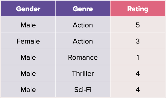
In this case, we would end up with the following equation (assume no bias and assume some encoding being done to categorical variables):
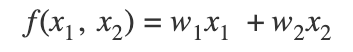
We would then solve for the weights w1 and w2. Naturally, the linear regression wouldn’t perform well because it tries to learn the average behaviour of each variable and does not take into account the possibility of interaction between these variables (i.e. it cannot learn that x1 may have a correlation with x2).
Poly2
To model these interactions, we introduce the next simplest model — Poly2. Instead of the above equation, we add in an interaction term for each feature pair. This gives us:
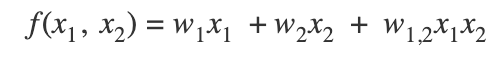
However, it is quite clear that there are some major downsides to this method. First, interactions that are very few will have an unreliable prediction and second, unseen interactions (i.e. zero interactions) will have trivial predictions.
For example, in a training set of 10000 examples, if we only have 2 examples of males watching thriller movies, our future predictions on males watching thriller movies will solely be based on those 2 training examples (i.e. the interaction term’s weight is determined by 2 data points). Furthermore, if our training set has no examples of females watching sci-fi movies (as in above table), the predictions made on those will be trivial and meaningless.
Matrix Factorization (MF)
In MF, we typically represent the data in a slightly different manner. Instead of encoding each variable as male or female and using the genre of the movie, we want to capture the interactions between user and item. Let’s look at our new data:
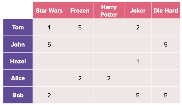
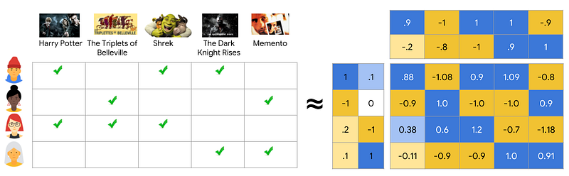
In the above diagram, users are placed in the rows while items are found in the columns. A positive value for a given user-item interaction is the rating that the user has given for that movie (note that values can also be binary as in below image to denote watched or not watched).
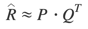
Given the user-item matrix above R [M x N], the goal is to approximate two matrices — a user latent matrix P [M x k] and an item latent matrix Q [N x k], where k is much smaller than N and M. The more robust method of MF is the weighted MF, where non-interaction values are populated with zeros and then optimized using weighted alternating least squares (WALS) or stochastic gradient descent (SGD) with the sum of squared errors (of observed and unobserved entries) as the loss function. A hyperparameter is usually added to weight the errors from the unobserved entries because they tend to be a lot more due to sparsity.
How is MF an improvement from Linear Regression and Poly2?
MF is inherently a latent factor model, meaning that it can represent a very sparse (and high-dimensional) matrix into two matrices that are much lower in dimensions. On a high level, one can imagine it in a similar way as principal component analysis (PCA), where we try to capture as much variance as possible in k components.
Note: The concept of latent vectors is synonymous to vector embeddings, where the idea is to learn a compact representation from a high-dimensional space.
A downside of MF is that it is simply a matrix decomposition framework. As such, we can only represent the matrix as a user-item matrix and unable to incorporate side features such as movie genre, language, etc. The factorization process has to learn all these from existing interactions. Hence, factorization machines are introduced as an improved version of MF.
(Since this article is focused on FFM, I will not delve into greater details of MF. To find out more, I highly recommend Google’s introductory course on recommender systems.)
Factorization Machines (FM)
As introduced earlier, FM is an improved version of MF. More specifically, FM is a more generalized predictor like support vector machines (SVM), but is able to estimate reliable parameters under sparsity [2]. To put it simply, FM is formulated as a linear model, with interactions between features as additional parameters (features). These feature interactions are done in their latent space representation instead of their plain format. It is represented mathematically as such:
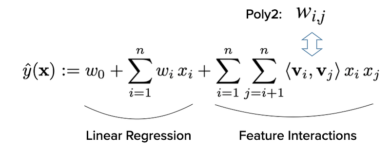
As mentioned, we can decompose the above equation into two parts — a Linear Regression model on the left-hand side and an equivalent matrix factorization on the right-hand side.
How are the interactions captured differently from Poly2?
The right-hand side of the above equation may scare people off because it does look intimidating. To understand it more easily, let’s take a look at how we can represent the user-item matrix we saw in MF.
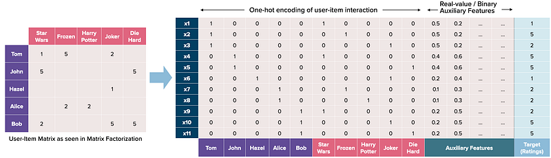
For a start, we want to represent the user-item interaction as a one-hot encoding vector, where each row of the transformed will only have a single active user and item. We can then add in auxiliary features (e.g. other movies the user has rated, last movie rated, time he consumed that movie, etc) either as one-hot encodings or normalized vectors.
Broadly speaking, factorization machines are able to estimate interactions in sparse settings because they break the independence of the interaction parameters by factorizing them (using latent vectors as expressed in <v_i, v_j>). This means that data for one interaction helps also to estimate the parameters for related interactions (similar to the idea of matrix factorization and collaborative filtering).
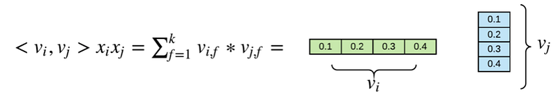
Compared to Poly2, the weights of each interaction in FM is estimated using the inner product of the two latent vectors instead. This means that even if there are no interactions between x_i and x_j in the training set, FM will be able to generalize this interaction because it has already created an embedding (as in MF example where we obtain two latent matrices) during training. In Poly2, this would not have been possible because the model has not seen this particular interaction. Note that in FM, there is an additional hyperparameter k — the number of latent features used (as seen in above diagram).
If FM can already generalize so well, how does FFM improve over FM?
Field Aware Factorization Machines (FFM)
Before delving into FFM, it is crucial to note the difference in terminologies: the independent variables such as Genre and Gender will now be termed fields. The categorical values that each field takes will be termed features. For example, male, female, action, romance, etc are all features.
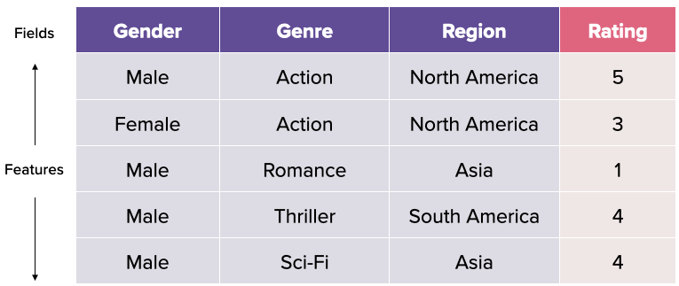
In FM, every feature has only one latent vector to learn the latent effect with all other features [1]. For example, if we have 3 fields Gender, Genre and Country, we would compute the interaction under FM as:

Taking the first row of the above table as an example, the latent vector of Male is used to learn the latent effect with Action <v_male, v_action> and North America <v_male, v_northamerica>. However, Action belongs to the Genre field while North America belongs to the Region field, yet we are using the same latent vector to represent Male.
FFM breaks down this single representation into multiple latent vectors — one to represent each other field. The intuition behind doing so is that the latent vector for <v_male, v_action> and <v_male, v_northamerica> is likely to be quite different and we want to capture them more accurately. The interaction under FFM would then be as follows:

To learn the latent effect of <v_male, v_action>, we use v_male,genre because we want to use the latent vector specifically for the genre field. Likewise, we use v_action,gender because we want to capture the latent vector specifically for the gender field.
When should we use FFM over FM?
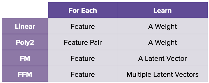
Comparing FFM versus FM, FFM learns multiple latent vector for each feature while FM learns a latent vector for each feature. One can interpret the former as trying to represent the interactions in a more granular-level. As such, the number of latent features k needed to represent such granular interactions is lesser i.e. k in FFM << k in FM.
In the official FFM paper, it is empirically proven that for large, sparse datasets with many categorical features, FFM performs better. Conversely, for small and dense datasets or numerical datasets, FFM may not be as effective as FM. FFM is also prone to overfitting on the training dataset, hence one should use a standalone validation set and use early stopping when the loss increases.
Summary
Hope this was helpful to anyone who is exploring the use of FFM or FM in the application of supervised learning with sparse matrices or exploring recommender systems. :) Feel free to leave comments!

Support me! — If you like my content and are not subscribed to Medium, do consider supporting me and subscribing via my referral link here (NOTE: a portion of your membership fees will be apportioned to me as referral fees).
References:
[1] Field Aware Factorization Machines for CTR Prediction
[3] Google’s Recommender System Course
[4] Thrive and blossom in the deep learning: FM model for recommendation system (Part 1)


