

An Introduction to Regression Discontinuity Design
conduct reliable causal inference with historical data
A causal relationship, unlike a correlation, is a much stronger relationship between two variables. Although it is hard to claim a causal relationship, it gives meaningful insights and informative guidance once proven. In my previous article, I have discussed what, why and how regarding causal inference:
As mentioned in the article, the most reliable way of demonstrating a causal relationship is through running random trials, which are also known as experiments. However, it is not always feasible to conduct randomized trials. In this case, we could use some “tricks” widely applied in economic research to conduct causal inference with historical data. Regression Discontinuity Design (RDD) is one of these tricks when certain conditions apply. In this article, I will show you what RDD is and some applications using RDD for causal inference.
Why not experiment?
Randomly assigning control and treatment groups ensures no significant difference between the two groups except the treatment effect, thus identifying a causal relationship without worrying about confounding variables. Conducting an experiment is the most reliable method to analyze causal relationships, but it’s not the most common way mainly due to two reasons:
- It is costly to run experiment: running randomized trails is not only financially costly but also time-consuming. It is hard to run field experiments without solid budget invested in the project;
- It is not always applicable to run experiment: There are a lot of reasons that makes running experiments not feasible. For example, it is not ethnical to run experiments on some medical treatments. Plus, sometime it is impossible to assign subjects into treatment and control groups without worrying the interactions between the two groups, especially when running experiments on social media.
If it is not possible to generate new data through experiments to conduct causal inference, the other solutions are applying special methodologies on historical data. Depending on the scenarios and the assumptions, we can choose from Regression Discontinuity Design (RDD), Difference in Differences (DID), Instrument Variables (IV), Propensity Score Matching (PSM), etc. In this article, I will elaborate on the assumptions and applications with Regression Discontinuity Design.
What is RDD?
One challenge of using historical data for causal inference is that we can never know the true counterfactual outcome, meaning that we never know what would have happened if a subject in the treatment group was assigned to the control group, or vice versa. Thus the outcome difference we observe from simply comparing the treatment and control group is not the true treatment effect, but can be biased by other variables. All the methodologies for causal inference involve finding reliable ways to estimate the true counterfactual effect. For randomized trails, utilizing randomness, we ensure subjects in the two groups are the same in every aspect except receiving treatment or not. In propensity score matching, we “match” the comparison between treatment and control group subjects based on their matching scores in some characteristics.
Regression Discontinuity Design measures the treatment effect at a cutoff, thus we can only apply RDD if there is a clear cutoff that separates the treatment and control group. This can be a natural cutoff such as a geographical border, or an intervention like a grade requirement for qualifying scholarship. By only comparing subjects locating closely on either side of the cutoff, we can estimate the average treatment effect and claim causal relationship.
The intuition behind RDD is that although we know there are bias for subjects to be assigned to different groups, we believe subjects who locate close to the cutoff are quite alike, and randomness is the only reason they are assigned into treatment or control group. It is quite similar to randomized trials but only with historical data.
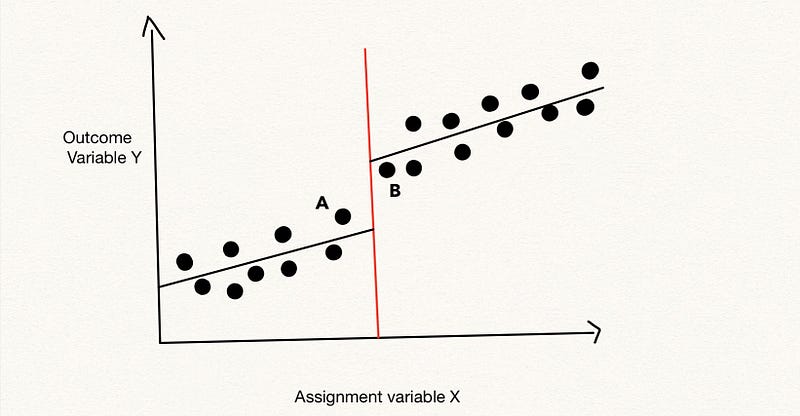
Just as the graph above shows, there is a discontinuity when plotting the regression between the outcome variable of our interest Y, and the assignment variable X (the variable with the cutoff) before and after the cutoff. The discontinuity exists both due to the treatment effect and other pre-existence differences among the subjects in treatment and control groups. However, we believe for subjects who are close to the cutoff c, like A and B, their outcome difference mostly comes from the treatment because they are very close to each other in terms of the X variable.
Applications in RDD
RDD was first applied to evaluate the effect of a scholarship program (Thistle and Campbell 1960). If we want to know the impact of receiving scholarships (the treatment) on students’ future grades (the outcome variable), simply comparing the grades for students with and without scholarships will induce bias into the estimation. Students who receive scholarships because of their past grades may score higher than other students even without the scholarship! The simple comparison would overestimate the treatment effect. However, if we only focus on students near the cutoff grade for giving scholarship, i.e. students who almost got the scholarship (slightly lower than the cutoff), and students who barely got the scholarship (slightly higher than the cutoff), we can estimate their future grades differences and claim causal relationships. Since these students have their past grades so close to each other, we believe they are quite alike in every aspect except receiving scholarships or not, that is exactly what we needed for causal inference.
Another interesting application is to use RDD to estimate Uber customer’s price elasticity and demand curve using historical transaction data (Cohen et al(2016)). Price elasticity describes the causal relationship between quantity purchased by customers and the prices they are facing. Customers with high price elasticity are sensitive to price change. Simply regress price and quantity purchased from the historical transaction data would induce bias from other factors that also affect customers’ purchasing decisions, like seasonality, customer incomes, etc. In this paper, the researchers take advantage of Uber’s “surge” pricing algorithm and conduct a regression discontinuity design to estimate demand elasticities at several points along the demand curve. The intuition is that during “surge” price, the algorithm will endogenously generate a surge multiplier based on the local market supply and demand conditions, customer characteristics, etc. Even though the surge multiplier is endogenous with the market conditions, there are some levels of randomness that can be useful to estimate price elasticity. The market conditions between surge multipliers “1.244” and “1.246” are quite similar to each other, however, since the surge multiplier is only in two digits, the former leads to “1.24” while the latter leads to “1.25”. Since the market conditions are quite similar for customers near the cutoffs, by estimating the differences in reactions (transactions) from customers near the cutoffs, they are able to estimate price elasticity and the demand curve by each point.
Although RDD is a good way of estimating casual relationship with historical data, that doesn’t mean that we cannot utilize it to create new data for the sake of casual inference. Just as the Uber example demonstrates, incorporating certain levels of randomness in the algorithm can help you analyze causal relationship later on. Plus. it is much cheaper than running field experiments sometimes.
Caveats
Although RDD provides a convenient method to estimate causal relationship, we still need to check carefully whether the assumptions apply before jumping into the analysis:
- The subjects should not affect whether they can receive the treatment: In the scholarship example, students shouldn’t be able to convince the professor to give them scholarship even their grades failed to pass the cutoff;
- The cutoff should not be contaminated by treatments that share the same cutoff: For example, the fact that the legal access to gambling is also at 21 could contaminate a study analyzing the impact of alcohol using RDD and the cutoff at 21.
That is all for this article. Thank you for reading. Lastly, don’t forget to:
- Check these other articles of mine if interested;
- Subscribe to my email list;
- Sign up for medium membership;
- Or follow me on YouTube;
- Watch my most recent YouTube video about How much Have I Made Writing at Medium:
Reference
[2] Lee, David S., and Thomas Lemieux. 2010. “Regression Discontinuity Designs in Economics.” Journal of Economic Literature, 48 (2): 281–355.
[3] Thistlethwaite, D. and D. Campbell. “Regression-discontinuity analysis: An alternative to the ex post facto experiment.” Journal of Educational Psychology 51 (1960): 309–317.
[4] Cohen, P., Hahn, R., Hall, J., Levitt, S., & Metcalfe, R. (2016). Using big data to estimate consumer surplus: The case of Uber (No. w22627). National Bureau of Economic Research.


