Amazon Fashion Discovery Engine (Content-Based Recommendation)

Real-world problem

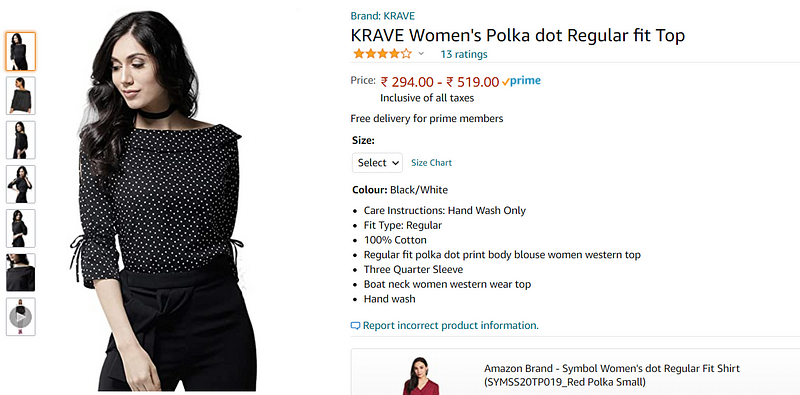
Whenever we visit amazon.com, this is our product image. We have multiple images of the same product.
“Krave” is the brand name.
“KRAVE Women’s Polka dot Regular fit Top” is the title. The title has a lot of interesting and important information.
Below the title, we have the price,size,colour and then product description.

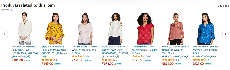
Then it shows related/similar products in terms of our search.

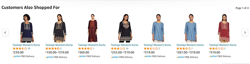
It also shows us “customer also shopped for” products which are also recommendations.
Why care about product recommendations? It is estimated that around 35% of the revenues that amazon makes are because of product recommendations. Due to product recommendation bars, as shown above, the user ends up buying a product or two.
Amazon internally uses two types of recommendation systems: 1) Content-Based Recommendation: When we search about polka dot shirts, it uses text and images to recommend similar products. 2) Collaborative filtering based Recommendation: Imagine, User U1 browsed through products i1,i2,i3 User U2 browsed through i1,i3,i4 Then I can recommend User U3, the product i3 when he is on page i1. So, this is called a collaborative filtering-based recommendation. Unfortunately, we don’t have this data.
So, in our case study, we will use content-based recommendations.

Plan of Attack

Setup python
Data Acquisition
Data cleaning
Text-Preprocessing
Linear Algebra
Text-based product recommendations -BoW -Word2Vec -Tf-IDF
Image-based product recommendation
A|B Testing

Amazon Product advertising API

I actually used Amazon’s own product advertising API as we need to obtain data from amazon.com using any programming language of our choice in a policy-compliant manner.

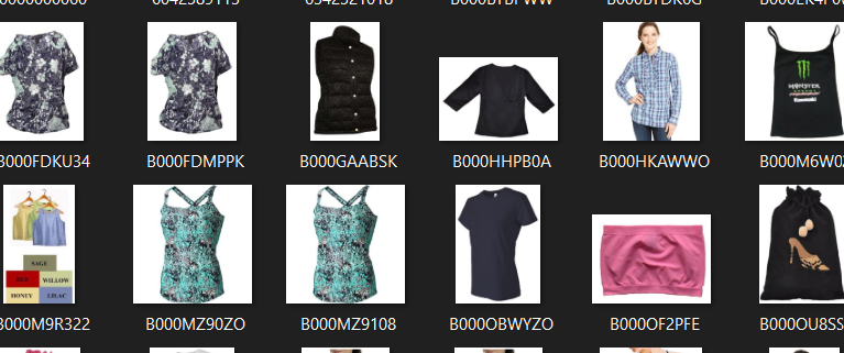
I obtained data on women’s tops and shirts and got data of roughly about 183000 products. We got data like Image-URL, Title, Price, Product Description, etc. So we will primarily focus on the data of women’s tops.

Overview of the data and the Terminology

Dataset is a set of data points.
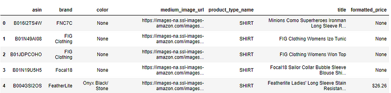
A row here represents a product in this dataset which is also known as data point.
Each column represents a variable/feature of a given product. For ex: It can have a price, title, imageURL etc.
Number of data points/products: 183138
Number of features/variables: 19

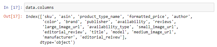
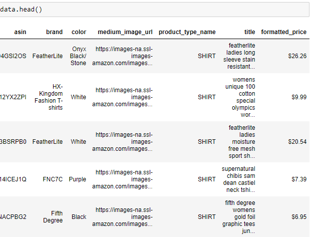
I will be using only 6 features out of these 19 features in this workshop. — 1. asin (Amazon standard identification number)- A unique no given to each product at amazon.com. — 2. Brand (brand to which the product belongs to) — 3. color (color information of apparel, it can contain many colors as a value , for ex: black and blue stripes) — 4. product_type_name (type of the apparel, ex: SHIRT/TSHIRT ) — 5. medium_image_url (URL of the image) — 6. title (title of the product) — 7. formatted_price (price of the product)
I have intentionally not used description as it is lengthy and takes longer time to process.

Well, some part of the feature drop comes from various EDA techniques and some from domain expertise. It’s sometimes Intuitive too.

Data Cleaning & Understanding

This is extremely important step in machine learning which is often overlooked. The better we understand our data, the more better models we can build. If we don’t want our models to suffer, let’s focus.

Here we can notice that, there are certain cells where data is missing or it is none. So let’s understand our data.

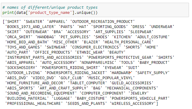
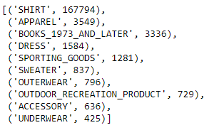
Basic stats for feature: product_type_name

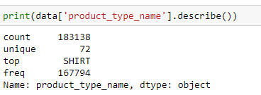
Out of 183138 products, 72 products are unique.

Top most product type found is “SHIRT”, which is present in 167794 out of 183138 that is roughly 91%.
The 10 most frequent product_type_names:

2. Basic stats for feature: brand

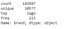
As in the data, out of 183138 products, brand name is given only for 182987 products. So there are 151 missing values.
There are 10577 unique brands.
The top most brand is “Zago” and is present in 223 rows.
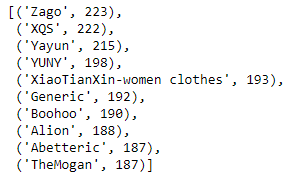
The top 10 brands are:

3. Basic stats for feature: color

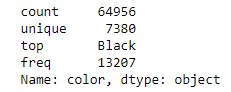
64956 products out of 183138 products have color information. That’s approximately 35.4%.
There are 7380 unique colors.
The top most color is black and is found in 13207 products, which is 7.28% of the products.

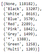
For 118182 products, color is not specified at all.

4. Basic stats for feature: formatted_price

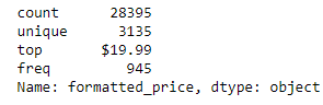
Only 28395 products out of 183K have information about price, which is roughly about 15.5%.
There are 3135 unique price points.
The top most price point is $19.99 and is present for 945 products.

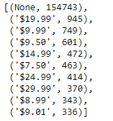
So, price value is missing for lot of the products and other look sensible.

5. Basic stats for feature: title

Titles are short and very informative.
They are one of the most important feature and we will use it extensively.

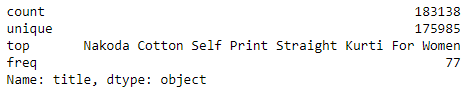
They are mostly present for every product, which makes it the best feature.

So, instead of operating on 183K data points, I will be operating on a subset of data points by removing those rows where some data is empty. As operating on 183K dataset is quite computationally expensive and time taking, so we will operate on a subsetof it.

6. Remove rows where formatted_price is null

I removed those rows in the dataset, where formatted_price was null or where price information was not given. I used logical not operation here to find all the formatted_price fields which are not null and stored them in data.

data = data.loc[~data['formatted_price'].isnull()]
print('Number of data points After eliminating price=NULL :', data.shape[0])

Number of data points After eliminating price=NULL : 28395

7. Remove rows where color is null

In the similar way, I removed those rows in the dataset, where color was null or any information about color of the product was not given. I used logical not operation here to find all the color fields which are not null and stored them in data.

data =data.loc[~data['color'].isnull()]
print('Number of data points After eliminating color=NULL :', data.shape[0])

Number of data points After eliminating color=NULL : 28385

We brought down the number of data points from 183K to 28K. Those who have time and no computational problem, please feel free to run this case study on 183K dataset.

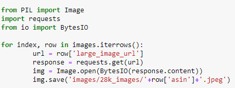
You can download all these 28K images using this code below. You do not need to run this code anyway unless if you want to download the images too. I have commented this code snippet in my code.

How would we deal with too many NULL values where imputations is hard and the column like price is too important to be dropped ? In such case we will take all the rows without price=null as train data.The rows where price=null is considered as test data. So, we train the model using train data and predict the price for test data as it’s price was null. Now instead of imputation we can replace the null values with the predicted values. There is a another easy way which says fill all the null values with “0”.

Remove Duplicate Items/Products

Remove duplicates : part 1

We have about 28K product at this time.
We need to find the number of products that have duplicate titles or exactly same title. As we know title is one of the most important feature and it is short and informative.

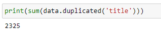
So 2325 products out 28K products have duplicate titles.

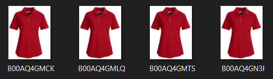
Here we can observe these products/Shirts are exactly same in color except different in size maybe(S,M,L,XL). Let’s say, the first image is the query product and we have to find similar products. If we recommend these exact shirts as query product of just different size to the customer , then it leads to bad customer experience because titles are exactly same.
So to avoid bad customer experience, we will remove duplicates.

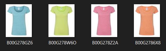
We can even have example of duplication where products are exactly same but different in color. When one of these images is the query product, it’s not always best to recommend different color product of the same product.
So, in our data there are many duplicate products like the above examples, we need to de-dupe them for better results.

Remove duplicates : part 2

I will remove all products with very few words in title. So if the length of the title is greater than 5, then I will consider it, otherwise I will remove it.

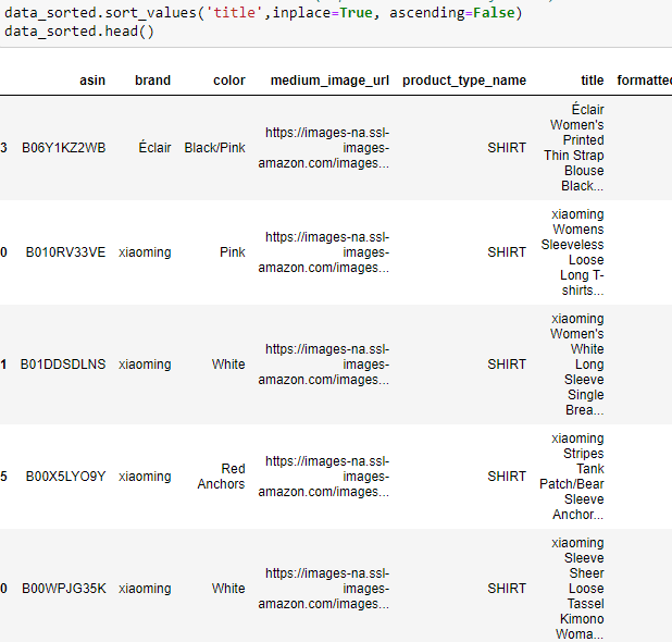
After removal of products with short description: 27949

Now, I will sort the whole data based on title (alphabetical order of title) in the descending order.

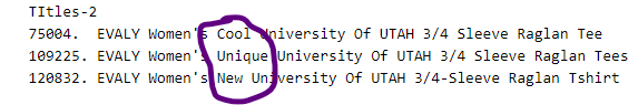
Some examples of duplicate titles that differ only in the last few words/suffix.

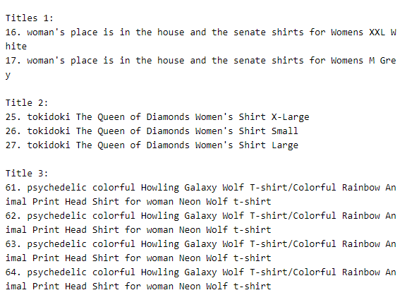
As these titles are sorted alphabetically, we can get these similar titles with just different last few words consecutively. So we will this logic.

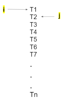
Let’s say I have my variable “i” here and my variable “j” here at (i+1). Since they are already sorted, I will compare how many words does my ith title and jth title differ in. The way I can do this is, I can pull all the words of T1 in a set and all the words of T2 in a set and carry out set difference between them. If the difference is less than 2, then we will consider those two titles as similar and remove the duplicate which differ only at the end. So we will remove T2 and then increment “j” and keep doing it. Once we compare T1 with everything else. Then again I will increment my “i” to T3 and “j” to (i+1) place. We will keep doing this till the end of for loops.

Number of data points after removing the duplicates which differ only at the end :  17592

Remove duplicates : part 3

Previously, we sorted whole data in alphabetical order of titles. Then, we removed titles which are adjacent and very similar title.

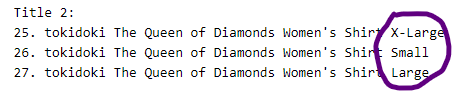
But there are some products whose titles are not adjacent but very similar.

These titles are exactly same except that one word that differs and cannot be solved sorting it alphabetically. So how do we remove them ? i: 1 → n j: 1 → n For every pair of (i,j): we will find out how many words they differ in. If difference of words in (Title i, Title j) is ≤ K words (let’s say), then we will remove Title j.

As we know, n = 17K products now, so how many pairs can I form now ? → nC2 =n(n-1)/2 →17KC2= 17592(17592–1)/2 = 154730436 = 154 Million So, we need to carry out 154 Million title pairs compairision.

Number of data points after stage two of dedupe:  16042

Text Pre-Processing: Tokenization and Stop-Word Removal

Stop word removal is a text pre-processing stage in NLP.
Stop words are a set of commonly used words in a language. Examples of stop words in English are “a”, “the”, “is”, “are” and etc. Stop words are commonly used in Text Mining and Natural Language Processing (NLP) to eliminate words that are so commonly used that they carry very little useful information.
I used the list of stop words that are downloaded from nltk lib.
I removed all the special characters in the title like ‘“#$@!%^&*()_+-~?>< etc.
I converted all letters to lower case.
I removed stop words from the titles.
In my system, it took me around 3.5 seconds to remove stop words from all the titles from the data.

Text Pre-Processing: Stemming

To put it simple, stemming is the process of removing a part of word or reducing a word to it’s stem or root which might not have meaning in dictionary.
Let’s assume we have a set of words: fishing, fisher, fished It’s root word is fish. Similarly for the set of words: arguing, argue, arguement It’s root word is argu.
I tried stemming our titles using porter stemmer, but it did not work very well. In the end, it’s all about experimentations.

So at the end of the pre-processing steps:

de-duped data
Removed stop-words

I am left with around 16K products as my dataset.

Now, let’s build our product similarity system based on text of titles.

Text based product similarity

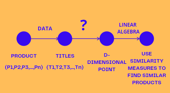
For every product, we have a title.
Given a title, How can we convert it into a d-dimensional point ? There are multiple ways to convert a text into d-dimensional point.
Given a d-dimensional representation of title,we can use similarity measures to find similar products.

Converting text to an n-D vector : bag of words(BoW)

S = Set of words which are present in any of the titles (T1,T2,T3,….,Tn). Let’s say this set S has size “d”, or d is size of unique words in S. d = no of unique words in S.
Now , I will be creating a d-dimensional vector for each title. Let’s say word1 in vocabulary/set is present 0 times in title 1, so we put value as “0” in the vector. Similarly word 4 is present 2 times in title 1, so we put the value as “2” in the vector.

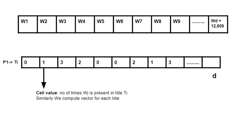
So in bag of words, I am excluding the sequence of the text or the sequence information. It is an extremely simple & powerful technique.

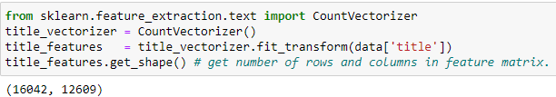
With literally executing these 3 lines of code, it gives us a matrix of 16042 rows and 12609 columns. For any title Ti, it can at most have 20 words out of 12609 unique words , so most of the cells in the matrix would be “0”. So in our case as most of them are zero, it’s useless to store memory locations of 16K x 12K cells. So we will store them in sparse matrix instead of 2-D array to solve the memory problem. In the above code, fit_transform returns sparse matrix.

Bag of Words based Product Similarity

Our function bag_of_words_model takes title id and no of similar products you want it to recommend as the parameters.
pairwise_dist will store the distance from given input apparel to all remaining apparels. The metric I used here is euclidian distance to measure distance between one title to another title.
np.argsort will return indices of the smallest distances of title feature.
pdists will store the smallest distances of title feature.
data frame indices also stored the indices of smallest distaces.
we will pass 1. doc_id 2. title1 3. title2 4. URL 5.model to the get_result function.
Now, we will call the bag-of-words model for a product to get similar products.

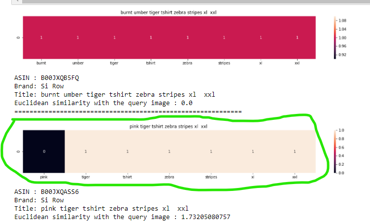
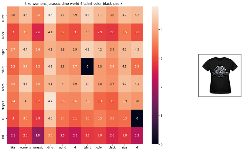
Let’s understand the visualization: heatmap Here it says, the word pink is not present in the query, that’s why it is “0”. The word tiger is present in query, so it is “1”. Similarly all other words are present in the query. The more pink it is or the more non zero values you have, the more closer both titles are or the more is the overlap. The color represents the intersection with the query/input title.

TF-IDF: featurizing text based on word-importance

Each of title is known as document and collection of document is known as document corpus.

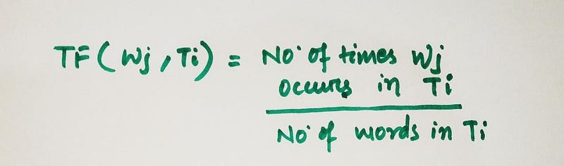
Term frequency means how frequently a term or word occurs in a document/title. If wj occurs multiple times in a title, then term frequency also increases.
IDF(Inverse Document Frequency): Given a document corpus and word j, it gives us natural logarithm of no of documents in the corpus by no of documents in the corpus that contains the word Wj.

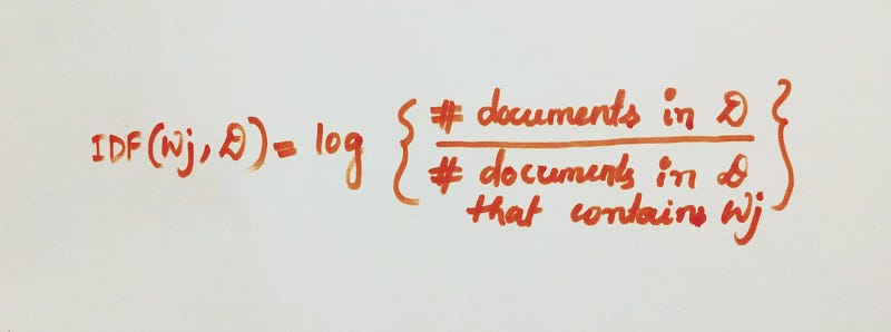
IDF(Wj) increases, if Wj is rare in document corpus. As the denominator decreases, the ratio increases and the log of the whole function increases.
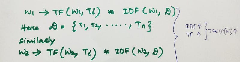
So, Tf-IDF now measures and evaluates how relevant a word is to a document in a collection of documents/corpus. TF-IDF is the product of term frequency and inverse document frequency. So if a word occurs a lot of times in a document but occurs rarely across all the titles in the corpus. then IDF will be high. So, this how we calculate TF-IDF vector for title Ti.

TF-IDF based Product Similarity

Our function tfidf_model takes title id and no of similar products you want it to recommend as the parameters.
pairwise_dist will store the distance from given input apparel to all remaining apparels. The metric I used here is euclidean distance to measure distance between one title to another title.
np.argsort will return indices of the smallest distances of title feature.
pdists will store the smallest distances of title feature.
data frame indices also stored the indices of smallest distaces.
we will pass 1. doc_id 2. title1 3. title2 4. URL 5.model to the get_result function.
Now, we will call the tfidf_model for a product to get similar products.

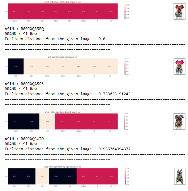
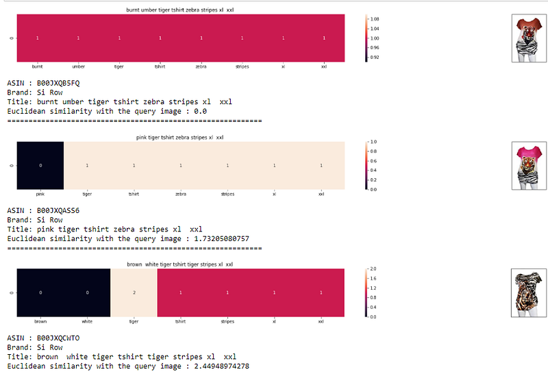
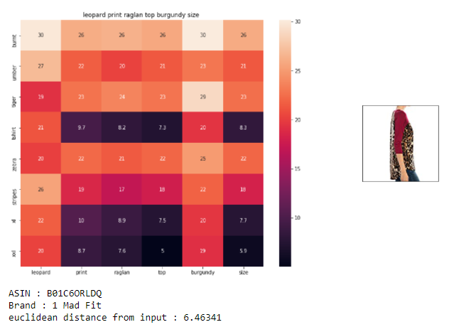
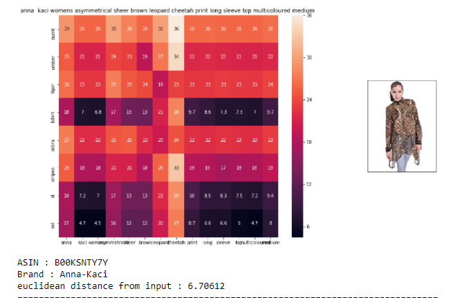
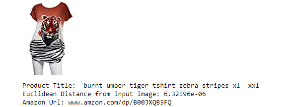
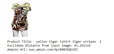
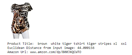
For ex: “burnt” is a rare word, tf-idf value for burnt is high and since burnt belongs to the query title, the other product with title that has “burnt” word will be similar to our query image. Now, those two titles will be similar because, burnt word is a rare word, so IDF is high which leads to high tfidf value. Here similarity is calculated based on tfidf values.
Now rare words like “burnt” and “umber” will have very similar kind of tfidf values, let’s say 0.2 and 0.3 respectively. In that case distance between them will be small and thus more chance of getting recommended.
So, we have a better chance of getting better recommendations than similarity based on bag of words.
Since “burnt” has higher tfidf value, so we end up getting such burnt color top recommendation too.

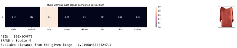
So bag of words was just using frequency of words, while tfidf is using rarity and importance of words which pops out to be quite a really nice technique for recommendation.

IDF based Product Similarity

In this case study, If we observe the titles:

Words don’t repeat often.
There are variations in titles, as there are longer and shorter titles.
Term frequency(TF) for shorter titles are high. In that case, tfidf will prefer shorter titles.
So in our case, term frequency would have made sense if Ti is a web-page or a long document, because words that occur more often should be given importance. Here each title is hardly having 15 or 20 words, so it’s better to drop term frequency and use only IDF(Inverse document frequency).We can experiment it out and see for the results if it worked out better than tfidf or not.
To use IDF attribute only and ignore TF values, we fitted data using CountVectorizer and defined our own IDF function.
In our case it did not work out that well.

Text Semantics based product similarity: Word2Vec

Bag of words and tfidf do not account for semantics. Both were frequency based techniques and used to return sparse vectors.
Given title, we want it to convert it into d- dimensional array and use euclidean distance for finding similarity. But can we find semantic similarity ?
One such very popular technique is Word2Vec. It returns me an dense array or most of the cells are non zero. Word2Vec algorithm will observe pattern in our data corpus and give us a d-dimensional vector. Word2Vec typically requires very large data corpus.
Google has trained Word2Vec on google news corpus and for each word in this corpus we get 300 dimensional vector. Google has provided us this model free of cost. So we will use google news word2vec.

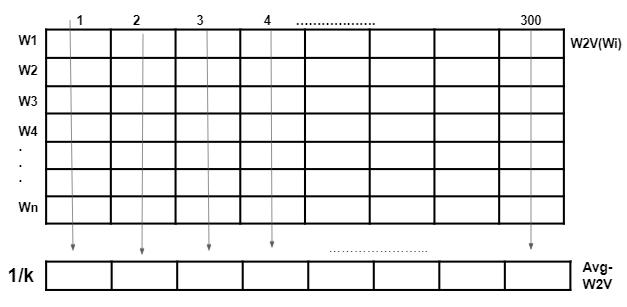
Let’s assume there are k words in our title Ti. To get word2vec of Ti, we take sum of all the first components of all words, similarly keep adding components of all cells till 300 dimension and get a new vector. I will then divide all the components of the new vector by k. This is known as average word2Vec of any sentence.

Average Word2Vec Product Similarity

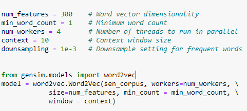
We can even build a custom Word2Vec using our own text data. Since we don’t have large corpus like google, we will just use google’s Word2Vec. For reference you can through this code. It’s that easy to build your own custom word2vec model if you have enough data. You need to set values for various parameters such as word vector dimensionality, minimum word count, number of threads to run in parallel, context window size etc. and then you can simply initialize and train your model.

Now if you have a RAM ≥ 12GB , then you can successfully use google vector file, because you will have vector for millions and millions of words and it will take a lot of time. If we recall, we had about 12,609 unique words. So instead of storing all the data of millions of words, why can’t we create a simple dictionary, where we can store/sample only our 12,609 words and their corresponding vectors. So this would save a lot of memory and I put it into a pickle file.
We can write down some utility functions to get word2vec, for computing distances and our heatmap function and a function for computing average Word2Vec for all the titles as explained before using build_avg_vec function.
Now we can build our avg_w2v_model just like every other model, where we find pair wise distances, sort and find nearest points.
we will pass 1. doc_id 2. title1 3. title2 4. URL 5.model to the get_result function and call the avg_w2v_model for a product to get similar products. Let’s check out, how w2v gives different result.

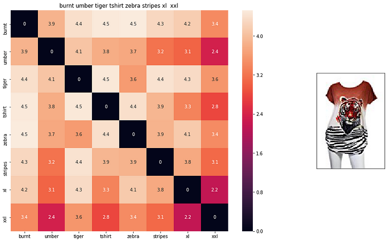
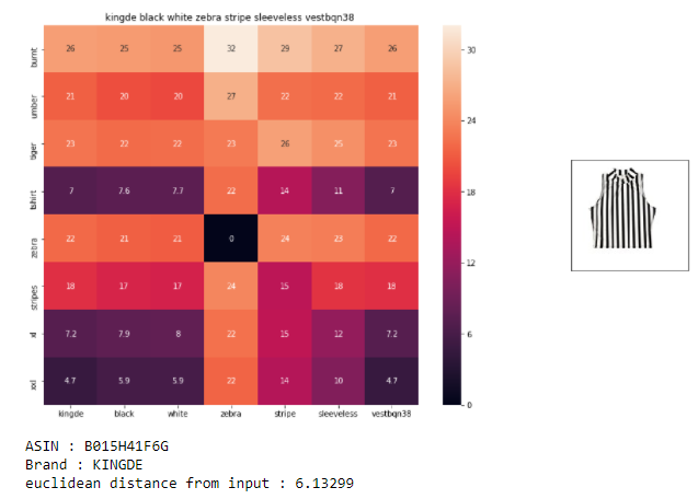
If you pick any value here, let’s say 3.6, it is the euclidean distance between word2vec of zebra and word2vec of tiger. Lower this value, more related these two terms. Just look at euclidean distance between xxl and xxl, as they both are same, so they have a value of “0”. So darker values are smaller values in the scale.

So word2vec gave us semantic similarity. I would suggest you must go through the code and all the visualizations to get the grasp of semantic similarity which was never captured by bag of words, tfidf.

TF-IDF Weighted Word2Vec based product similarity

In TF-IDF, we use word importance. Now if we leverage tfidf concept to combine with word2vec, then we have the potential of word importance as well as semantic similarity. This is known as TF-IDF weighted Word2Vec.
I have a document corpus of titles D = {T1,T2,T3,…,TN} Let’s say, Ti is having 5 words, k = 5 and Wi of Ti is a 300 dimensional vector. I already found TF-IDF(Wi,Ti,D) of this word Wi in the title Ti of the corpus D. Now, whatever value of TF-IDF I get, I multiply it with each component of 300 dimensional array of Wi. Similary I carry out the process with all the words of Ti with their respective TF-IDF’s. Then I will find N = sum of all TF-IDF values of all words in Ti.
we take sum of all the first components of all words, similarly keep adding components of all cells till 300 dimension and get a new vector similar to average word2vec. I will then divide all the components of the new vector by N. This is known as TF-IDF Weighted Word2Vec of any sentence.

IDF weighted Word2Vec based product similarity

Instead of computing TF-IDF, we can only compute IDF weighted Word2Vec. IDF also gives us word importance in our corpus because if a word occurs few times then it is given higher importance and word2vec gives us semantic similarity. I have not used term frequencies with word2vec in my code because titles are small and most words occur only once.
The code is very similar to what we did earlier. So you can go through the code on my github repo. We find pair wise distances, pass some parameters and find similar products.

We successfully got some really interesting similar products based on query which other models did not give. IDF weighted Word2Vec gave us amazing results.
As of now we have seen different techniques like BoW, TF-IDF, avgw2v, IDF weighted w2v and every technique had a fair result. But from a business perspective and impact, how to decide, which model is the best ? We will understand A|B testing to get to that.

Weighted Similarity Using Brand & Color

Till now, we have just used titles for product similarity. We have not used brand and color yet. These are the additional variables, that we can leverage.
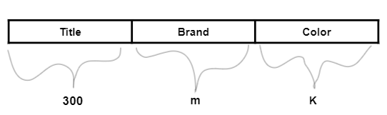
For each product Pi, we already got title vector. Similarly for each product Pi, we will get brand vector and color vector. Once we get these 3 vectors, we will concatenate these vectors.
Let’s say, I have m no of brands. Let’s assume, product bi has brand bi, How do I write it as a vector ?

So this will be a m dimensional vector. The value corresponding to the cell which is the brand is let’s say ith index value. Only ith index value in the vector will be “1” , rest all the cells will have “0” as the value. Such an encoding is called one hot encoding.
Similarly, we will carry out one hot encoding for colors too.
Now after concatenating, I have a vector where part of the vector is representing title, part of the vector is representing brand and part of the vector is representing color.

Given two products, pi and pj, I can simply find euclidean distance between pi and pj using this full vector.
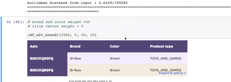
Let’s assume, we want to prefer showing our customers products of the same brand or same color. So, can I modify my euclidean distance to somehow incorporate this preference ? All we have to do is to take weighted euclidean distance. We have to construct three weights : weights for title (Wt), weights for brand (Wb), weights for color (Wc). Then you multiple each of the elements of title vector with Wt, each of the elements of brand vector with Wb and each of the elements of color vector with Wc. After you multiply, you just take the euclidean distances
For ex: if Wt = 1, Wb = 5, Wc = 1, as we have given more weight to brand, so we end up preferring products of same brand. More the weight, more is the preference.
The selection of weight is dependent a lot on the domain knowledge and it’s the role of a data scientist to tune the values of weight and see what works better.
Let’s look at the results:

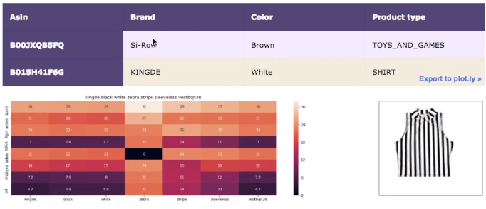
Here, brand and color are completely different from the query, still it pops up because we gave same weight of 5 and 5 to brand and color.

Here we are giving more weight to brand and color.

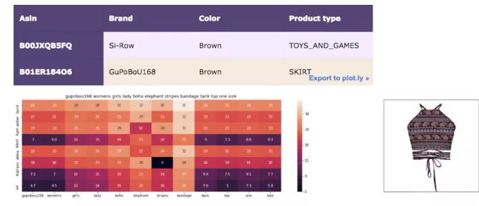
We can observe here, that as the brand changes, but the color stays brown. Even if one changes, the other one compensates because we have given equal weight of 50 to brand and color.

So these are the strategies which we can incorporate in our recommendation system.

Building a real world solution

We worked on Bag of words based product similarity model. We worked on TF-IDF based product similarity model. We worked on IDF based product similarity model. We worked on Word2Vec based product similarity model. We worked on Average Word2Vec based product similarity model. We worked on TF-IDF Weighted Word2Vec based product similarity model. We worked on IDF Weighed Word2Vec based product similarity model. We worked on Weighed Similarity using brand and color based product similarity model.
So , we worked on multiple techniques. But, How does real world solution/system built ? Most companies use multiple techniques.

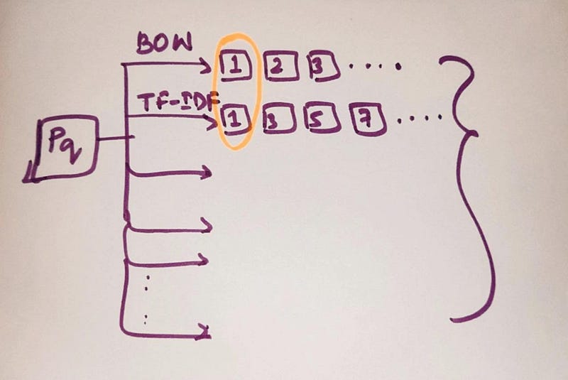
All these results are taken into consideration and we combine all these results. Since product “1” is occurring a lot of times, even though I am using different algorithms and same result pops up. Probably that result is very important. So, I will apply business rules.
Business rules can be like : - Do not show the products of same brand more than twice or thrice. - The product manager can make similarly more such rules and finally we get a final list of products. - These bunch of business rules test the quality of results.
The final list that I get will be shown to customer.
Now, how do we know if our solution is good ? For that, there is A|B testing which is also known as live testing or Bucket testing.

Deep learning based visual product similarity

ConvNets: How to featurize an image: edges, shapes, parts

For every product Pi, I have an URL to image. From this URL, I can download the product image. Now how do I convert my image into a d-dimensional vector ?
We can extract various features from the image like edges, shapes, colors, pattern like zebra stripe, leopard print etc. What if given an image and we can construct a vector. A part of the vector would be about color, a part of the vector would be about shapes and a part of the vector would be about pattern or edges. Now I can use euclidean distance to find distance between two vectors.
So, given an image, I will use convolutional neural networks like VGG-16 to convert my image into dense vector. If two images are very similar, then euclidean distance between vector 1 of image 1 and vector 2 of image 2 will be very small.
We will use some existing CNN’s which is VGG-16 for our task to build image based product similarity.VGG-16 takes an image and converts it into a 25,088 dimensional dense vector.
All my images are of length (224,224) and I have about 16,042 samples.
The important function save_bottlebeck_features has 3 parts. The first part basically builds the VGG-16 network. The generator part takes each of my images and run through the VGG-16 network and returns me the 25,088 dimensional features. I also collect asins name for each of my product. At the end, I am doing a numpy save, I am saving my 16K images converted into CNN vector features into .npy files along with the asin names.
Remember, here we include top = false, so it won’t include the last fully connected layers and hence the output won’t be 1000. The last conv layer in VGG-16 gives an output of shape 512 x 7 x7. On flattening this output we will get 25,088 length vector.
Now we will use euclidean distance to find similarity. I will simply load the image features for the 16K images and their corresponding asins names. I will load the original 16K dataset, where I have title , brand, color, URL , type of each product.Now we will get similar products using CNN features of VGG-16.
I define the function “get_similar_products_cnn” and pass the parameters such as image id and number of similar results for the query I want. Just like our any previous models, I find my pairwise distances and also find the nearest points. I will just call the function and get similar products.

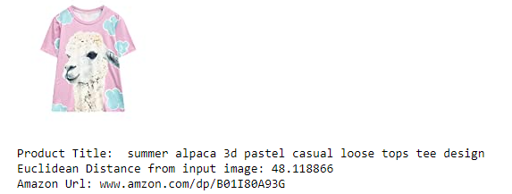
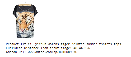
Here, It will only uses the image to find similar products.

If you observe, these products are very similar. Based on the query image, the model is focusing more on tiger prints and zebra stripes.

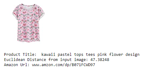
This product was not available at all previously for the same query title. So, we are getting some new varieties of recommendations similarities.

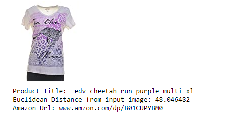
I just use the images to find similarity, but I am still getting very good results. In the above product recommendation, we got cheetah image as well as zebra stripes, which is quite a good recommendation without title. We did not get this product in any of the approaches in text based similarity.

So, we got some really interesting results out of deep learning. In real world we combine solutions from multiple approaches.

Measuring goodness of our solution: A|B testing

Through out the blog, I kept evaluating our approaches on the basis of single query which is incorrect. But in real world, we will be dealing with millions of images or titles or products. So, how do you evaluate solution and solution 2 ?
Let’s assume the ellipse is the set of all users that visit amazon.com. Millions of users visit amazon.com daily. I just randomly split my users into two non overlaping groups: let’s say U1 and U2. For users in Set U1, I will show them results of solution 1 and results of solution 2 to the users of Set U2. They are roughly similar sets. Now, I measure my sales on Set 1 and measure my sales on Set 2. If sales(U1) > sales(U2), then users tend to prefer solution 1 more than solution 2. So company will prefer solution 1.
So, for evaluation, we have to carry out A|B testing to measure the goodness of our solution by checking the sales.
The other day, I was going through a video of an amazon engineer who says after the model goes into production, it usually takes a month to get all feedback of the model performance.

Conclusion

Recommender system can help the user to find the right product.
It increases the user engagement.
In Amazon, 35% of the products get sold due to recommendation.
It helps to make the content more personalized.

The implementation is available on my GitHub page:

GitHub - Swetadas-1718/Amazon-Fashion-Discovery-Engine-content-based-recommendation

It is estimated that around 35% of the revenues that amazon makes are because of product recommendations. Due to…

github.com