AM broadcasting, audio transmission simulated in Python

This article continues the series of articles about the AM modulation. AM technique has been simulated previously, but only for tone signals. The AM modulator and a simple demodulator have been analyzed in this article, while more demodulated have been studied here. Now, a more complex and more realistic data signal is used, audio signals. This article presents the Python code to simulate the AM modulation and demodulation of audio signals. AM broadcasting was the first technique used to transmit audio signals and it is still used nowadays. Finally, the simulation results are used to conclude the advantages and disadvantages of the AM modulation.

Python simulation

Two different simulations in Python have been carried out. Firstly, the modulation and demodulation of an audio signal is presented. This simulation shows how the demodulation process gets a recognizable signal. Then, simulations with noise added to the received signal is shown. Results show the susceptibility of the AM modulation to noise.

AM Modulation & Demodulation

First of all, we import the required libraries. We will use the NumPy, SciPy and Matplotlib:

import numpy as np
import matplotlib.pyplot as plt
from scipy.signal import butter,filtfilt,normalize,resample
from scipy.io import wavfile

Then, the audio file is read, you can find example wav files online. The scipy.io.wavfile function returns the audio samples, as well as the sampling frequency. The AM modulator has been codified for mono signals, so be sure that you are using mono audio. For stereo audio, you have to get only one of the audio channels. Furthermore, audio samples are normalized to work with a signal which runs from -1 to +1 values.

fs, data = wavfile.read('input_file.wav')
data = data[:,0]                       # ONLY FOR STEREO AUDIO
# normalize signal
max_data = max(abs(data))
data = data/max_data

We still need to do some adaptation to the signal before modulation. To ensure the Nyquist theorem after modulating, we must increase the sampling frequency. Otherwise, there would be aliasing for the carrier signal, whose frequency is higher than the modulator signal (our audio signal). To solve this, an upsampling of the audio signal is carried out. As an example, an upsampling factor of 10 is selected. For the typical sampling frequency in audio, which is 44.1kHz, this upsampling gives us a final sampling frequency of 441kHz. Afterwards, the AM modulation signal is generated. In this case, a carrier frequency of 80kHz has been selected.

# Upsampling
up_factor = 10
data_2 = resample(data, up_factor*len(data))
fs2 = up_factor*fs

# AM Modulation
A_c = 1                     # Carrier amplitude
f_c = 80e3                  # Carrier frequency
m = 0.7                     # Modulation index

t_max = len(data_2)/fs2
t = np.linspace(0, t_max, (int)(t_max*fs2))
carrier = np.cos(2*np.pi*f_c*t)
am = (A_c+A_c*m*data_2)*carrier

In the receiver side, a synchronous demodulator is used, since we already saw in this article that this is the best option. The code to simulate the synchronous receiver (adapted to our AM modulator) is:

# Synchronous rx

mixer_out = am*carrier

fc = fs/2
b, a = butter(5, fc/(fs2*0.5), btype='low', analog=False)
modulator_rx_synch = filtfilt(b,a,mixer_out)
modulator_rx_synch = modulator_rx_synch-np.mean(modulator_rx_synch)

Finally, we only need to save the received sound to play with our music player. If you reproduce the output file, you can recognize the original sound, even AM modulation distorts the signal a little bit.

modulator_rx_synch = (modulator_rx_synch*max_data).astype(np.int16)
wavfile.write("output_file.wav", fs2, modulator_rx_synch)

Take into account that the sampling frequency to save the file is fs2, which will be typically 441kHz. At this point, we can resample the signal to the original sampling frequency (fs) again before saving. However, to check the proper working of the AM modulation and demodulation process we can use fs2.

AM Modulation & Demodulation, noise effects

In wireless telecommunication systems, there are always unwanted signals which are called noise. This noise is any modification that the signal suffers in the wireless channel. The most common noise in a wireless system is the Additive White Gaussian Noise (AWGN), which is modeled as a random signal which follows a zero-mean normal distribution. The random signal is added to the signal.

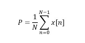
An important measure which shows the quality of the received signal in terms of noise is the Signal to Noise Ratio (SNR), which is the ratio between the signal power and the noise power. The higher the SNR the higher the quality. The following expression is used to compute the power of any signal:

Also, for a random signal distributed as a zero-mean normal distribution, the variance of is the power.

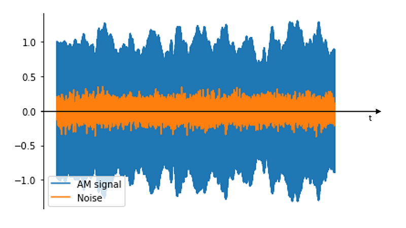
In the simulation, the AM signal has a power which depends on the audio signal. However, for the above parameters, the signal power will be a little bit higher than 0.5. This is due to the fact that the carrier power is 1/2. The following code generates a noise whose power is 0.01 and adds it to the signal:

# Noise
noise_power = 0.01
mean = 0
std = np.sqrt(noise_power)
noise = np.random.normal(mean, std, size=len(am))

# Signal + noise
am_rx = am+noise

This results in a signal power 50 times higher than the noise power, that is, the SNR is 50. Typically, the SNR is measured in dB, so in this case we have a SNR of 17dB. Both data and noise signals are represented below to show the difference between them.

Finally, we demodulate again and save the result, getting the audio when an AWGN channel is modeled. If we hear the audio now, we realize how this noise affects the signal. Even the SNR is quite high, we can hear the white noise in our audio. This is an intrinsic problem of the AM modulation, and it is due to the fact that the noise is added to the amplitude of the signal. Therefore, the noise is directly affecting the data signal.

Advantages and disadvantages of AM modulation

The main advantage of the AM modulation is its simplicity. As it have been seen in this simulations, both the modulator and the demodulator are quite simple and they can be done by a circuit having few components. As a results, this technique is really cheap.

However, the problem of AM modulation is its low robustness against noise. This simulation shows how the data is directly affected by the noise, even for a high SNR. Also, as we seen in this article, the AM modulation and demodulation process adds to the signal some distortions. This is the reason why AM gave way to other audio broadcast techniques, such as FM modulation.

References

• Steven A. Tretter, https://user.eng.umd.edu/~tretter/commlab/c6713slides/ch5.pdf
• Rick Lyons, https://www.dsprelated.com/showarticle/938.php
• https://en.wikipedia.org/wiki/Additive_white_Gaussian_noise

Have you spent your learning budget for this month, you can join Medium here:

Other articles you may find interesting: