AlphaZero, a novel Reinforcement Learning Algorithm, in JavaScript

Learn about and implement AlphaZero, entirely in JavaScript!

In this blog post, you will learn about and implement AlphaZero, an exciting and novel Reinforcement Learning Algorithm, used to beat world-champions in games like Go and Chess. You will use it to master a pen-and-pencil game (Dots and Boxes) and deploy it into a web app, entirely in JavaScript.

AlphaZero’s key and most exciting aspect is its ability to gain superhuman behavior in board games without relying on external knowledge. AlphaZero learns to master the game by playing against itself (self-play) and learning from those experiences.

We will leverage a “simplified, highly flexible, commented, and easy to understand implementation” Python version of AlphaZero from Surag Nair available in Github.

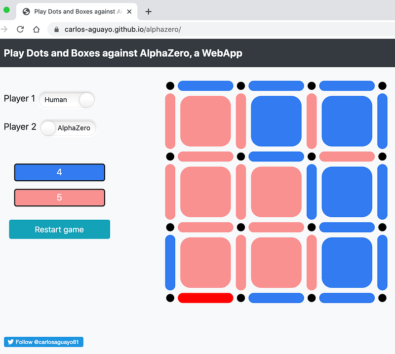
You can go ahead and play the game here. The WebApp and JavaScript implementation are available here. This code was ported from this Python implementation.

https://carlos-aguayo.github.io/alphazero/

AlphaZero is described in the paper bySilver, David, et al. “Mastering the game of Go without human knowledge” nature 550.7676 (2017): 354–359.

Dots and Boxes game

Dots and Boxes is an elementary child’s game with a surprising level of complexity in it.

Two players take turns to place a horizontal or vertical line between two adjacent dots. The player who completes the fourth side of a 1×1 box scores one point and gets another turn. The game ends when the board is full, and the player with the most points wins.

Artificial Intelligence and Board Games

We have pondered for a long time if machines can demonstrate intelligence. How to validate the machine’s ability to exhibit intelligent behavior? A typical way has been playing board games, like Chess, and attempting to gain superhuman behavior to defeat world champions.

In 1957, Herbert Simon predicted that a computer system would beat the world chess champion in ten years. It took much longer than that, but in May 1997, a computer defeated the Chess world champion, Garry Kasparov.

Despite the remarkable milestone, one can argue whether this computer system was “intelligent”.

These computer systems are composed of three elements:

1. Human-defined Evaluation Functions.
2. Game tree search algorithms.
3. Very powerful hardware.

The evaluation function would take the board as an input and return the board’s “value”. A high value indicates a very favorable position for the current player. For example, a chessboard configuration where the player is about to do Checkmate would have a very high value.

Game tree search algorithms (like Minimax) search across all possible moves looking for the one that would guarantee a path to a board configuration with a high value. The search can be made efficient by not visiting configurations where we know that we won’t find a better value. That’s what Alpha–beta pruning does.

Finally, add very powerful hardware, and you would have a machine capable of defeating a world champion.

What’s the catch? Experienced players manually craft these evaluation functions. These systems would rely on openings books indicating the best-known moves. The middle game would use evaluation functions created by studying games from grandmasters. Then grandmasters would further fine-tune them.

For example, we could create an Evaluation Function for the Dots and Boxes game. A reasonable and straightforward evaluation function would be to compare the score. The higher the positive delta in the score, the more favorable the board game is. In most cases, that would work. However, in the Dots and Boxes game, like in many board games, the best moves can involve sacrificing in the short-term to have better gains in the long-term. In the Dots and Boxes game, sometimes it’s better not to score a box to avoid gaining another turn, and instead, force the move back to the opponent. We would then have to tune our evaluation function to consider an increasing number of complex scenarios!

The evaluation function that defeated Kasparov had 8,000 features! And the large majority of those features were created and tuned by hand!

So, without belittling an important milestone like defeating a chess world champion, an undesirable aspect was the need to have top-ranked players define these computers’ behavior and manually tweak so many variables.

What’s AlphaZero, and why is it so exciting?

AlphaZero is the first computer system capable of gaining superhuman behavior at games like Chess or Go, defeating world champions, bootstrapped with only the game’s rules and without human domain knowledge.

Given only the rules of the game, AlphaZero would start playing against itself. Learning, little by little, strategies and techniques, gaining relatively quickly superhuman behavior.

Whereas systems like DeepBlue would require chess experts’ assistance, AlphaZero would become strong by playing against itself. Furthermore, AlphaZero showed superhuman strength not only in Chess but also at Go. Go is a more complicated game for computers, given its much larger game space and other factors.

While humankind has accumulated knowledge in games like Go and Chess from millions of games played over thousands of years, AlphaZero, a straightforward algorithm using only the game rules, rediscovered this knowledge and new strategies in a few days.

There’s even a movie about it.

How would AlphaZero learn with just self-play?

Recall that systems like DeepBlue would rely on a human-defined “evaluation function”, which would take as an input the board state and output the “value” of the state.

Nowadays, it’s extremely easy for DeepLearning models to take as an input an image and classify it as a dog or a cat. The idea is to take the board as the input to a DeepLearning model and train it to predict if the board has a winning or losing configuration.

But to train a Machine Learning, one needs data, lots of data. Where do you get a dataset of games? Simple, we let the computer play against itself, generating a set of games and make a dataset out of it.

AlphaZero training algorithm

The algorithm is straightforward:

1. Let the computer play against itself several games, recording the board at every move. Once we know the outcome, update all those boards with the given result, “win” or “lose” at the end of the game. We have then built a dataset to give to a Neural Network (NN) and start learning if a given board configuration is a winning or losing one.
2. Clone the Neural Network. Train the clone using the dataset generated in the previous step.
3. Have the clone and original Neural Network play against each other.
4. Pick whatever Neural Network wins, drop the other one.
5. Go to step 1.

And just like magic, after many iterations, you have a world-class model. This model managed to outperform the strongest computer chess program in only 4 hours!

AlphaZero components

AlphaZero has two components. We already talked about the first one, which is the Neural Network. The second one is the “Monte Carlo Tree Search” or MCTS.

1. Neural Network (NN). Takes as input the board configuration and outputs the board’s value, plus a probability distribution for all the possible moves.
2. Monte Carlo Tree Search (MCTS). Ideally, the Neural Network would be enough to choose the next move. We still want to look at as many board configurations as possible and ensure that we are indeed picking the best possible action. MTCS is, like Minimax, an algorithm that will help us look at board configurations. Unlike Minimax, MTCS will help to explore the game tree efficiently.

Let’s dive into details and determine the next move

It’s easier to follow AlphaZero by first looking at its behavior when determining the next move (competitive mode) and then look at the training routine.

Neural Networks (NNs) are already great at classifying things, like a cat versus a dog. The idea here is simple, can the Neural Network learn to classify a board configuration as a winning versus losing one? More specifically, the Neural Network will predict a value expressing the probability of winning versus losing. Furthermore, it will output a probability distribution over all the possible moves, representing which action we should explore next.

The Neural Network takes the game state as an input and outputs a value and a probability distribution. Specifically for Dots and Boxes, the game state is represented by three elements: First, whether a line has been played or not, using an array of 0 and 1’s for each line across dots. 1 if a player has already colored the line, else 0. Second, if the current move is a pass, third, the score. We can represent all the required information with these three elements to determine a board’s value and predict its next move.

Let’s analyze the following game, where it’s the Blue player’s turn. Blue has two options, follow the top path and lose, or play the bottom path and win.

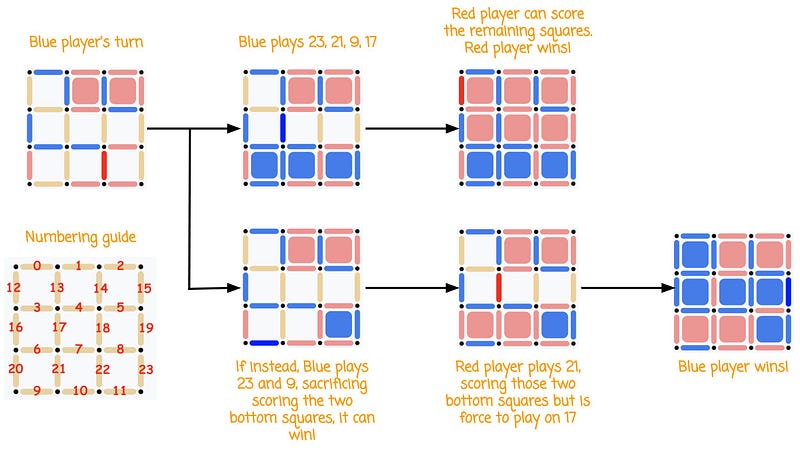
If Blue plays 23 followed by 21, Red wins. Instead, if Blue plays 23 followed by 9, Blue wins. How would AlphaZero find the winning move if it would be playing Blue?

You can reproduce the results seen below by using this notebook.

If we feed that board configuration to the Neural Network, we get an array with move probabilities for each action:

move_probability[0]: 9.060527501880689e-12
move_probability[1]: 3.9901679182996475e-10
move_probability[2]: 3.0028431828490586e-15
move_probability[3]: 7.959351400188552e-09
move_probability[4]: 5.271672681717021e-11
move_probability[5]: 4.101417122592821e-12
move_probability[6]: 1.2123925357696643e-16
move_probability[7]: 6.445387395019553e-23
move_probability[8]: 2.8522254313207743e-22
move_probability[9]: 0.0002768792328424752
move_probability[10]: 1.179791128073232e-13
move_probability[11]: 5.543385303737047e-13
move_probability[12]: 3.2618200407341646e-07
move_probability[13]: 4.302984970292259e-14
move_probability[14]: 2.7477634988877216e-16
move_probability[15]: 1.3767548163795204e-14
move_probability[16]: 8.998188305575638e-11
move_probability[17]: 7.494002147723222e-07
move_probability[18]: 8.540691764924446e-11
move_probability[19]: 9.55116696843561e-09
move_probability[20]: 4.6348909953086714e-12
move_probability[21]: 0.46076449751853943
move_probability[22]: 2.179317506813483e-20
move_probability[23]: 0.5389575362205505
move_probability[24]: 5.8165523789057046e-15

We also get a value for the board configuration:

-0.99761635

You can find the code that generates these values here.

There are a few interesting things from these outputs:

1. The highest probability moves are 23, 21, and 9, out of the 8 possible moves. If the NN plays 23 or 21, he scores a point. 23 is the winning move and has a slightly higher value (0.53) than the 21’s (0.46).
2. The NN will output probabilities even for invalid moves. It’s the code’s job to follow the game rules and ensure that we don’t play an invalid action.
3. The value is -0.99. That indicates that AlphaZero thinks that it has lost the game. The value ranges from -1 (loss) to 1 (win). This value should have been much closer to 1 (win) than -1 (loss) as we know that this is a winning state. Perhaps we need more training rounds to get to a state where AlphaZero would learn the correct value for this board configuration.

It’s tempting to take the Neural Network’s outputs and decide our next move.

In board games (and in life!), players typically see many “moves ahead” when determining their next move. It’s no different here. We use our Neural Network predictions to choose which state to explore next and ignore the ones with low value. Like Minimax, traditional AI game tree search algorithms are inefficient because they have to analyze every single move before going into the next move. Games with even small branching factors make their game space intractable. The branching factor is the number of moves possible. The number of possible moves changes as the game progresses. If so, you calculate an average branching factor. Chess’s average branching factor is 35. Go’s is 250.

This means that, in Chess, just after two moves, there are 1,225 (35²) possible board configurations, whereas, in Go, it would be 62,500 (250²). In Dots and Boxes, for a 3x3 game, the initial branching factor is 24 and decreases with every move (unless it is a pass). So in the middlegame, when the branching factor is 15, there are 2,730 (15*14*13) board configurations after just three moves.

Instead, the NN will guide us and tell us where we should explore and avoid being overwhelmed by many useless paths. The NN is telling us that 23 and 21 are strong moves.

It’s the job of the Monte Carlo Tree Search to do that.

Monte Carlo Tree Search (MCTS)

The Neural Network has given us an indication for the likely next moves. The Monte Carlo Tree Search algorithm is the one that will help us traverse the nodes to choose the next move to make.

Take a look at this link for the paper’s graphical description of Monte Carlo Tree Search.

The way that MCTS works is that for a given board, it will run N simulations. N is a parameter of our model. At the end of these simulations, the next move will be the most visited. You can follow along with the code here.

An MCTS simulation consists of traversing down the game tree, starting from the current board, by selecting the node with the highest “Upper Confidence Bound (UCB)” value (defined below) until we reach a game state that we have not visited before, which is called a “leaf”. This is what the paper refers to as Part A, “Select”.

What’s UCB? It’s Q(s,a) + U(s,a). Where “s” is the state, and “a” is the action. Q(s,a) is the expected value that we expect to get from that state “s” following the action “a”, the same one from Q-Learning. Remember that in this case, the value will have a range from -1 (loss) to 1 (win). U(s, a) ∝ P(s, a) / (1 + N(s, a)). This means that U is proportional to P and N. Where P(s, a) is the prior probability for the tuple (s, a), the value returned by the NN, and N(s, a) is the number of times that we have visited the state s and taken action a.

# Upper Confidence Bound
ucb = Qsa[(s,a)] + Ps[s,a] * sqrt(Ns[s]) / (1 + Nsa[(s,a)]

The point of the UCB is to initially prefer actions with high prior probability (P) and low visit count (N), but asymptotically prefer actions with a high action value (Q).

You can follow the code along here.

Once a leaf is found, we run that board through the NN. This is what the paper calls Part B, “Expand and evaluate”. You can follow along with the code here.

Lastly, we will propagate back up the value returned by the NN. That’s what the paper calls Part C “Backup”. You can follow along with the code here.

Determining the next move

Let’s see how AlphaZero determines the next move for the state mentioned above.

AlphaZero will run 50 Monte Carlo Tree Search Simulations.

You can reproduce the results seen below by using this notebook.

These are the paths that follow at each iteration:

Simulation #1 -> Expand root node
Simulation #2 -> 23
Simulation #3 -> 21
Simulation #4 -> 9
Simulation #5 -> 17
Simulation #6 -> 12
Simulation #7 -> 19
Simulation #8 -> 3
Simulation #9 -> 18
Simulation #10 -> 23,24
Simulation #11 -> 21,24
Simulation #12 -> 23,24,21
Simulation #13 -> 21,24,23,24
Simulation #14 -> 23,24,9
Simulation #15 -> 23,24,17
Simulation #16 -> 21,24,9
Simulation #17 -> 23,24,12
Simulation #18 -> 23,24,18
Simulation #19 -> 21,24,17
Simulation #20 -> 23,24,21,24,9
Simulation #21 -> 21,24,19
Simulation #22 -> 23,24,3
Simulation #23 -> 21,24,18
Simulation #24 -> 23,24,19
Simulation #25 -> 21,24,23,24,17
Simulation #26 -> 23,24,21,24,18
Simulation #27 -> 23,24,21,24,3
Simulation #28 -> 21,24,3
Simulation #29 -> 23,24,21,24,19
Simulation #30 -> 21,24,12
Simulation #31 -> 23,24,21,24,9,24
Simulation #32 -> 21,24,23,24,12
Simulation #33 -> 23,24,21,24,9,24,18
Simulation #34 -> 21,24,23,24,9,24,17
Simulation #35 -> 23,24,21,24,9,24,12
Simulation #36 -> 23,24,21,24,9,24,3
Simulation #37 -> 21,24,23,24,9,24,19
Simulation #38 -> 23,24,21,24,9,24,18,17
Simulation #39 -> 21,24,23,24,9,24,18,17,24
Simulation #40 -> 23,24,21,24,9,24,18,17,24,19
Simulation #41 -> 21,24,23,24,9,24,18,17,24,19,24
Simulation #42 -> 23,24,9,21
Simulation #43 -> 23,24,9,18
Simulation #44 -> 23,24,9,17
Simulation #45 -> 23,24,9,19
Simulation #46 -> 23,24,9,12
Simulation #47 -> 23,24,9,21,24
Simulation #48 -> 23,24,9,3
Simulation #49 -> 23,24,9,21,24,18
Simulation #50 -> 23,24,9,21,24,17

The above means the following: In the first simulation, we haven’t seen that board before and thus is a “leaf” node and “expands” it. Expands means that it evaluates that board with the NN.

Simulation #1 -> Expand root node

In the second simulation, we have already expanded the root node so it’s no longer a “leaf” and so we can search for the node with the highest UCB

The action with the highest UCB is 23. It dives into that state, given that it has not seen that state before, and thus it’s a leaf node, it expands it, and the second simulation completes.

Simulation #2 -> 23

In this case, the NN gives a losing value for 23. We discussed this before. The NN could use even more training to learn that it’s indeed a bad state. But for now, this still works, as we will see below.

For the next simulations, at each time, the option with the highest UCB are the remaining options. That’s because after visiting each action, it finds out that it has a low value and, thus, a low UCB.

Simulation #3 -> 21
Simulation #4 -> 9
Simulation #5 -> 17
Simulation #6 -> 12
Simulation #7 -> 19
Simulation #8 -> 3
Simulation #9 -> 18

For the next simulations, an exciting pattern starts surfacing. Remember that the winning sequence is 23, 24 (skip), 9.

Simulation #10 -> 23,24
Simulation #11 -> 21,24
Simulation #12 -> 23,24,21
Simulation #13 -> 21,24,23,24
Simulation #14 -> 23,24,9
Simulation #15 -> 23,24,17
Simulation #16 -> 21,24,9
Simulation #17 -> 23,24,12
Simulation #18 -> 23,24,18
Simulation #19 -> 21,24,17
Simulation #20 -> 23,24,21,24,9
Simulation #21 -> 21,24,19
Simulation #22 -> 23,24,3
Simulation #23 -> 21,24,18
Simulation #24 -> 23,24,19

In simulations 10 through 24, the MCTS is already focusing its attention on nodes 21 and 23. This makes sense as with either of those two paths, we score a point.

Simulation #33 -> 23,24,21,24,9,24,18
Simulation #34 -> 21,24,23,24,9,24,17
Simulation #35 -> 23,24,21,24,9,24,12
Simulation #36 -> 23,24,21,24,9,24,3
Simulation #37 -> 21,24,23,24,9,24,19
Simulation #38 -> 23,24,21,24,9,24,18,17
Simulation #39 -> 21,24,23,24,9,24,18,17,24
Simulation #40 -> 23,24,21,24,9,24,18,17,24,19
Simulation #41 -> 21,24,23,24,9,24,18,17,24,19,24

Then in simulations 33 through 41, it starts going deep in the losing combination. Notice an interesting thing. Despite going deep, it never reaches the end of the game as there are still playable moves.

Simulation #42 -> 23,24,9,21
Simulation #43 -> 23,24,9,18
Simulation #44 -> 23,24,9,17
Simulation #45 -> 23,24,9,19
Simulation #46 -> 23,24,9,12
Simulation #47 -> 23,24,9,21,24
Simulation #48 -> 23,24,9,3
Simulation #49 -> 23,24,9,21,24,18
Simulation #50 -> 23,24,9,21,24,17

Then, in simulations 42 to 50, with the NN’s help, it realizes that 23, 24, 21 or 21, 24, 23 are not good options and focus entirely on the winning sequence 23, 24, 9.

After 50 simulations, our time is up, and we need to choose a move. MCTS chooses the move that we visited the most. Here are the number of times that we visited each move (on the first play):

counts[3] = 1
counts[9] = 1
counts[12] = 1
counts[17] = 1
counts[18] = 1
counts[19] = 1
counts[21] = 15
counts[23] = 28

Actions 3, 9, 12, 17, 18, and 19 are visited only once in the first 10 simulations. Then the MCTS focused on moves 21 and 23. Visiting action 23 for the last 9 simulations. Given that we visited action 23 the most, 28 times, MCTS returns that as the next move.

What are the takeaways?

1. Through each simulation, the MCTS will rely on the NN to follow the path that seems the most promising, using a combination of the accumulated value (Q), the move prior probability (P) given by the NN, and how often it has visited the node. Or, in other words, the path with the highest UCB.
2. During each simulation, the MCTS will go as deep as it can until it reaches a board configuration that it hasn’t seen before, and it will rely on the NN to evaluate the board to tell how good that board is.

If we compare it with classical approaches like using Minimax with Alpha-Beta Pruning and an Evaluation function, we can say the following:

1. In Minimax, the depth is a parameter established by the designer. It will go that deep and then use the evaluation function. Without Alpha-Beta pruning, it would have to visit all the nodes at the given depth, being very inefficient. In the above scenario, with 8 moves left, at depth 3, it would mean evaluating 336 boards. In MTCS, with 50 simulations, we only had to evaluate 50 boards and managed to go much deeper.
2. Alpha-Beta pruning would have helped us reduce the 336 number. However, it doesn’t allow us to follow an intelligent path.
3. We rely on the Neural Network to tell us the “value” of a board at all times rather than using a human-defined evaluation function.
4. It was interesting to see that the NN wasn’t predicting the right values at the initial moves. Nevertheless, it had the correct predictions as we got deeper without going all the way to the end of the game.
5. Lastly, notice the elegance and simplicity of AlphaZero. Whereas in Alpha-Beta pruning, you have to track an alpha and a beta parameter to know where to prune, and a human-defined evaluation function can be unwieldy. MCTS and NN make everything quite elegant and simple. You can follow all this in JavaScript!

Training the Neural Network

We are missing one last key aspect. How do we train the NN?

Luckily it’s straightforward. We mentioned the steps before:

1. Let the computer play against itself several games in “training mode”, recording the board at every move. Once we know the outcome, update all those boards with the given result, “win” or “lose” at the end of the game. We have then built a dataset to give to a Neural Network (NN) and start learning if a given board configuration is a winning or losing one.
2. Clone the Neural Network. Train the clone using the dataset generated in the previous step.
3. Have the clone and original Neural Network play against each other.
4. Pick whatever Neural Network wins, drop the other one.
5. Go to step 1.

What does it mean to play in “training mode”? The difference is a tiny one. When playing in “competitive mode”, we will always pick the move with the highest visit count. Whereas in “training mode”, for a certain number of moves during the beginning of the game, the counts become our probability distribution and encourage exploration. For example, let’s say that there are 3 possible actions and the visit count is [2, 2, 4]. In competitive mode, we would always pick the third action as it has the highest visit count. But in training mode, [2, 2, 4] becomes a probability distribution, 2+2+4 = 8 and thus [2/8, 2/8, 4/8] or [0.25, 0.25, 0.5]. In other words, we will pick the third action 50% of the time, whereas we will explore the first and second actions 25% of the time.

Then let’s use a simple Tic-Tac-Toe game to describe the dataset.

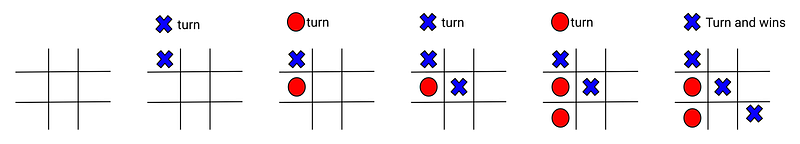
In the above game, the first player, the Xs win.

We can configure the board state by having zero if the square hasn’t been played, 1 if the first player, -1 if the second player has played the square.

For example, the board would be the following:

0 0 0    1 0 0     1 0 0     1 0 0     1 0 0     1 0 0
0 0 0 -> 0 0 0 -> -1 0 0 -> -1 1 0 -> -1 1 0 -> -1 1 0
0 0 0    0 0 0     0 0 0     0 0 0    -1 0 0    -1 0 1

Or:

[0, 0, 0, 0, 0, 0, 0, 0, 0]
[1, 0, 0, 0, 0, 0, 0, 0, 0]
[1, 0, 0,-1, 0, 0, 0, 0, 0]
[1, 0, 0,-1, 1, 0, 0, 0, 0]
[1, 0, 0,-1, 1, 0,-1, 0, 0]
[1, 0, 0,-1, 1, 0,-1, 0, 1]

Then we have to do two things. First, update each board as if it would be player1’s turn. We will always feed training data to the NN from the perspective of the first player. In TicTacToe, that’s simple. Every time it was the second player’s turn, we can flip the pieces to become player1’s perspective.

We go from this:

[0, 0, 0, 0, 0, 0, 0, 0, 0]  # Player 1 turn
[1, 0, 0, 0, 0, 0, 0, 0, 0]  # Player 2 turn 
[1, 0, 0,-1, 0, 0, 0, 0, 0]  # Player 1 turn
[1, 0, 0,-1, 1, 0, 0, 0, 0]  # Player 2 turn
[1, 0, 0,-1, 1, 0,-1, 0, 0]  # Player 1 turn
[1, 0, 0,-1, 1, 0,-1, 0, 1]  # Player 2 turn

To this:

[ 0, 0, 0, 0, 0, 0, 0, 0, 0]  # Player 1 turn
[-1, 0, 0, 0, 0, 0, 0, 0, 0]  # Player 1 turn 
[ 1, 0, 0,-1, 0, 0, 0, 0, 0]  # Player 1 turn
[-1, 0, 0, 1,-1, 0, 0, 0, 0]  # Player 1 turn
[ 1, 0, 0,-1, 1, 0,-1, 0, 0]  # Player 1 turn
[-1, 0, 0, 1,-1, 0, 1, 0,-1]  # Player 1 turn

Second, we append the game outcome. Let’s use a “1” if player 1 wins and “0” if it loses.

[ 0, 0, 0, 0, 0, 0, 0, 0, 0, 1]  # Winning board
[-1, 0, 0, 0, 0, 0, 0, 0, 0, 0]  # Losing board
[ 1, 0, 0,-1, 0, 0, 0, 0, 0, 1]  # Winning board
[-1, 0, 0, 1,-1, 0, 0, 0, 0, 0]  # Losing board
[ 1, 0, 0,-1, 1, 0,-1, 0, 0, 1]  # Winning board
[-1, 0, 0, 1,-1, 0, 1, 0,-1, 0]  # Losing board

The dataset is starting to get some shape! As you can see from the above, we can feed that to a NN to learn in a board is a winning or a losing one, the value.

We are missing the probabilities, though. Where do those come from? Remember that during training mode, we will still run MCTS simulations at every step. In the same way that we are recording the board configuration, we will record the probabilities.

We then clone the NN and train the clone using this dataset, expecting it to be slightly stronger as it’s using new data. We validate that it’s indeed stronger by having it compete against the original NN. If it wins more than 55% of the time, we consider it stronger and drop the original, and the clone becomes our new NN.

We keep repeating this process, and the NN will keep becoming stronger.

You can see the diagram from the paper here.

How come the dataset has stronger moves to learn from? By learning from the probabilities generated by the MCTS, they will usually select much stronger moves than the raw move probabilities given by the NN. We are feeding the NN knowledge obtained by having the MCTS go deep into many paths!

Use this notebook to train a Dots and Boxes model.

Deploying it into a WebApp

A few months ago, I published a blog post that walks you through the process of transforming a Keras or Tensorflow model into JavaScript to be used by Tensorflow.js. We are going to be doing the same here. We will convert the model we trained in Keras to be used in Tensorflow.js.

This notebook converts a pretrained Dots and Boxes model into a Tensorflow.js model.

Once we do that, we can easily load the model in JavaScript, as seen here.

Conclusion

In this blog post, you learned about AlphaZero, a novel Reinforcement Learning algorithm that can defeat world-champions in two-player, zero-sum board games.

You learned how it uses a Monte Carlo Tree Search along a Neural Network to find the best next move. You also learned how to train this Neural Network.

I hope that you enjoyed this blog post and found it valuable. If so, reach out!

I’m Senior Director of Software Development and Machine Learning Engineer at Appian. I’ve worked at Appian for the last 15 years, and I keep having a blast. This pandemic has not slowed us down, and we’re hiring! Send me a message if you would like to know how we craft software, please our customers and have fun!