AlexNet Explained: A Step-by-Step Guide

Guide to AlexNet: Architecture, Layers, and Practical Usage

AlexNet is a pioneering convolutional neural network (CNN) architecture that played a crucial role in popularizing deep learning, particularly for image recognition tasks. It was developed by Alex Krizhevsky, Ilya Sutskever, and Geoffrey Hinton, and it won the ImageNet Large Scale Visual Recognition Challenge (ILSVRC) in 2012 by a significant margin.

Alex Krizhevsky, Ilya Sutskever, and Geoffrey Hinton

You can find the original paper here.

AlexNet was essentially a successful implementation of ideas that had been around for decades, but it took advantage of technological advances in hardware and software that weren’t available when these concepts were first introduced.

The core idea behind AlexNet, the CNN, was not new. CNNs were first introduced by Yann LeCun and others in the late 1980s and early 1990s, most famously with the LeNet-5 architecture for handwritten digit recognition (e.g., the MNIST dataset).

LeNet: A Foundational Step in Deep Learning History

LeNet-5: Revolutionizing Image Recognition with Deep Learning

python.plainenglish.io

Although CNNs were well-known, they were too computationally expensive for large-scale data and deep networks. By the early 2010s, GPUs became affordable and powerful enough to train deep networks on large datasets like ImageNet, which AlexNet utilized extensively.

ImageNet contains over 14 million images categorized into 1,000 classes.

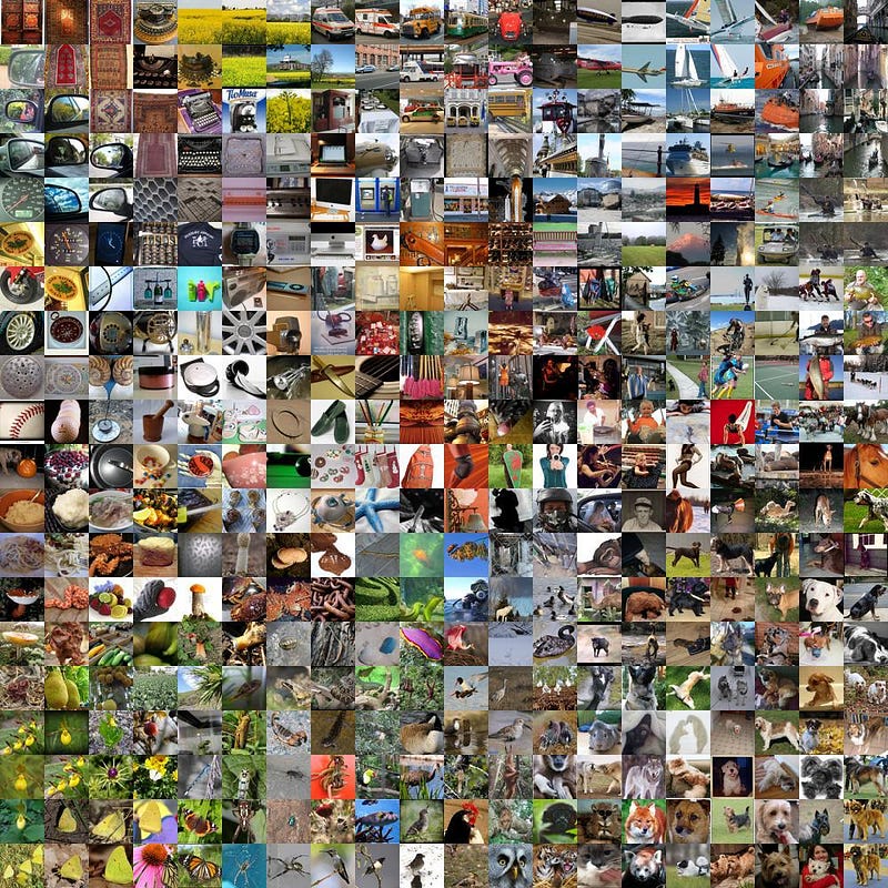
The ILSVRC 2012 subset (commonly used in classification tasks) has about 1,281,167 training images, 50,000 validation images, and 100,000 test images. It is available in Kaggle. It is around 167 GB.

The Architecture

The AlexNet architecture consists of eight layers: five convolutional layers followed by three fully connected layers.

INPUT LAYER: 227x227x3 (RGB image)

CONV1 (Convolutional Layer): Filter size is 11x11 with stride 4, no padding. There are 96 filters. (227 — 11)/4+1 = 55 -> The output size is 55x55x96 (96 feature maps of size 55x55, since there are 96 filters.

MAXPOOL1 (Max-Pooling Layer): It is an overlapping max-pooling layer. It means that the stride (in our case, it is 2) is smaller than the window size, causing the pooling regions to overlap.

Pooling window size is 3x3. (55–3)/2+1 = 27 -> The output size is 27x27x96 (96 feature maps of size 27x27)

CONV2 (Convolutional Layer): This time 256 filters with 5x5 size. Stride is 1 and padding is 2. (27+2*2–5)/1+1 = 27 -> The output size is 27x27x256.

MAXPOOL2 (Max-Pooling Layer): Again overlapping; 3x3 window size with 2 strides. The output is 13x13x256 (256 feature maps of size 13x13).

CONV3 (Convolutional Layer): 384 filters with 3x3 size. Stride and padding are 1. The output size is 13x13x384 (384 feature maps of size 13x13).

CONV4 (Convolutional Layer): This layer is similar to Conv3 but continues to refine the features learned from the previous layers.

CONV5 (Convolutional Layer): The final convolutional layer reduces the number of filters back to 256, which helps refine the extracted features before passing them to the fully connected layers. 3x3 size; stride and padding are 1.

MAXPOOL3 (Max-Pooling Layer): The final max-pooling layer reduces the spatial dimensions, preparing the data for the fully connected layers. Overlapping; 3x3 with 2 strides.

FC1 (Fully Connected Layer): 4096 neurons. After flattening the output from the convolutional layers, AlexNet passes the data through a fully connected layer with 4096 neurons. Plus Dropout.

FC2 (Fully Connected Layer): 4096 neurons.

OUTPUT LAYER FC3 (Fully Connected Layer): 1000 (one neuron for each class in the ImageNet dataset). The softmax activation function is used to output probabilities for each class, with the sum of probabilities equal to 1.

The model starts by receiving an RGB image resized to 227x227 pixels.

At the first layer, AlexNet uses large filters (11x11). Why? In the early stages, it’s essential to capture large-scale patterns, such as the rough shape and texture of objects. Think of these large filters as the network’s way of seeing the “big picture” — like the silhouette of an object — rather than focusing on fine details. The large stride (4) also quickly reduces the spatial size of the image, making computation more efficient.

By setting the pooling window size to 3x3 and the stride to 2, AlexNet ensures that the pooling regions overlap, meaning less information is lost during downsampling.

Now that the image is downsampled and large patterns are recognized, AlexNet adds more filters and uses smaller filters (5x5) in this layer. The network now focuses on more specific details, such as corners, edges, and textures, while preserving the same spatial dimensions through padding.

In the next convolutional layers, the filters get even smaller (3x3), but the number of filters increases dramatically (from 256 in Conv2 to 384 in Conv3 and Conv4). These layers specialize in learning abstract, high-level patterns, such as intricate textures, patterns, and small parts of objects (e.g., eyes, wheels).

AlexNet uses dropout in the fully connected layers, which randomly disables 50% of the neurons during training. This forces the network to learn more robust features and not rely too heavily on any one neuron.

In the final fully connected layer (FC3), AlexNet uses a softmax function to output probabilities for each of the 1000 classes in ImageNet. The class with the highest probability is chosen as the network’s prediction.

Python Code

I am going to repeat the implementation of this beautiful COLAB, from this Youtube video.

The dataset preparation:

import tensorflow_datasets as tfds

(train_dataset, test_dataset), info = tfds.load(
    'cats_vs_dogs',
    split = ('train[:80%]', 'train[80%:]'),
    with_info = True,
    as_supervised=True)

len(train_dataset), len(test_dataset)

for X, y in train_dataset:
  print(X.shape, y.numpy())
  image_1 = X.numpy()
  break

import matplotlib.pyplot as plt

plt.imshow(image_1)

import tensorflow as tf

def normalize_img(image, label):
  return (tf.cast(image, tf.float32) / 255.0, label)

def resize(image, label):
  return (tf.image.resize(image, (224, 224)), label)

train_dataset = train_dataset.map(resize, num_parallel_calls=tf.data.AUTOTUNE)
train_dataset = train_dataset.map(normalize_img, num_parallel_calls=tf.data.AUTOTUNE)

SHUFFLE_VAL = len(train_dataset) // 1000   # Divide by big value on free Colab
BATCH_SIZE = 4   # Use small batch size on free Colab

train_dataset = train_dataset.shuffle(SHUFFLE_VAL)
train_dataset = train_dataset.batch(BATCH_SIZE)

train_dataset = train_dataset.prefetch(tf.data.AUTOTUNE)

test_dataset = test_dataset.map(resize, num_parallel_calls=tf.data.AUTOTUNE)
test_dataset = test_dataset.map(normalize_img, num_parallel_calls=tf.data.AUTOTUNE)
test_dataset = test_dataset.batch(BATCH_SIZE)

test_dataset = test_dataset.prefetch(tf.data.AUTOTUNE)


for (img, label) in train_dataset:
  print(img.numpy().shape, label.numpy())
  break

The model structure:

from tensorflow.keras import layers
from tensorflow.keras.models import Model

def build_alexnet_model():
  inp = layers.Input((224, 224, 3))
  x = layers.Conv2D(96, 11, 4, activation='relu')(inp)
  x = layers.BatchNormalization()(x)
  x = layers.MaxPooling2D(3, 2)(x)
  x = layers.Conv2D(256, 5, 1, activation='relu')(x)
  x = layers.BatchNormalization()(x)
  x = layers.MaxPooling2D(3, 2)(x)
  x = layers.Conv2D(384, 3, 1, activation='relu')(x)
  x = layers.Conv2D(384, 3, 1, activation='relu')(x)
  x = layers.Conv2D(256, 3, 1, activation='relu')(x)
  x = layers.MaxPooling2D(3, 2)(x)
  x = layers.Flatten()(x)
  x = layers.Dense(4096, activation='relu')(x)
  x = layers.Dropout(0.5)(x)
  x = layers.Dense(4096, activation='relu')(x)
  x = layers.Dropout(0.5)(x)
  x = layers.Dense(1, activation='sigmoid')(x)

  model = Model(inputs=inp, outputs=x)

  return model

model = build_alexnet_model()
model.summary()

"""
Model: "model"
_________________________________________________________________
 Layer (type)                Output Shape              Param #   
=================================================================
 input_1 (InputLayer)        [(None, 224, 224, 3)]     0         
                                                                 
 conv2d (Conv2D)             (None, 54, 54, 96)        34944     
                                                                 
 batch_normalization (Batch  (None, 54, 54, 96)        384       
 Normalization)                                                  
                                                                 
 max_pooling2d (MaxPooling2  (None, 26, 26, 96)        0         
 D)                                                              
                                                                 
 conv2d_1 (Conv2D)           (None, 22, 22, 256)       614656    
                                                                 
 batch_normalization_1 (Bat  (None, 22, 22, 256)       1024      
 chNormalization)                                                
                                                                 
 max_pooling2d_1 (MaxPoolin  (None, 10, 10, 256)       0         
 g2D)                                                            
                                                                 
 conv2d_2 (Conv2D)           (None, 8, 8, 384)         885120    
                                                                 
 conv2d_3 (Conv2D)           (None, 6, 6, 384)         1327488   
                                                                 
 conv2d_4 (Conv2D)           (None, 4, 4, 256)         884992    
                                                                 
 max_pooling2d_2 (MaxPoolin  (None, 1, 1, 256)         0         
 g2D)                                                            
                                                                 
 flatten (Flatten)           (None, 256)               0         
                                                                 
 dense (Dense)               (None, 4096)              1052672   
                                                                 
 dropout (Dropout)           (None, 4096)              0         
                                                                 
 dense_1 (Dense)             (None, 4096)              16781312  
                                                                 
 dropout_1 (Dropout)         (None, 4096)              0         
                                                                 
 dense_2 (Dense)             (None, 1)                 4097      
                                                                 
=================================================================
Total params: 21586689 (82.35 MB)
Trainable params: 21585985 (82.34 MB)
Non-trainable params: 704 (2.75 KB)
_________________________________________________________________
"""

tf.keras.utils.plot_model(
    model,
    to_file='model.png',
    show_shapes=True,
    show_dtype=False,
    show_layer_names=False,
    show_layer_activations=True,
    dpi=100
)

Model architecture output. Image by author.

Training:

from tensorflow.keras.optimizers import Adam
from tensorflow.keras.losses import BinaryCrossentropy

model.compile(loss=BinaryCrossentropy(),
              optimizer=Adam(learning_rate=0.001), metrics=['accuracy'])

from tensorflow.keras.callbacks import EarlyStopping

es = EarlyStopping(patience=5, 
                   monitor='loss')

model.fit(train_dataset, epochs=100, validation_data=test_dataset,
          callbacks=[es])

We don’t need to train AlexNet whenever we need it. We can easily use a pre-trained AlexNet model in Python.

PyTorch contains pre-trained models, including AlexNet.

import torch
import torchvision.models as models
import torchvision.transforms as transforms

I will use an image to use in prediction from an URL.

import requests
from PIL import Image
from io import BytesIO

Let’s load the pre-trained AlexNet model, which has been trained on the ImageNet dataset. The evaluation mode is necessary for making predictions (inference).

# Load the pre-trained AlexNet model
alexnet = models.alexnet(pretrained=True)
alexnet.eval()

We define a series of transformations to preprocess the image before feeding it into the AlexNet model. These transformations ensure that the image has the correct format and size for the model.

# Defining the preprocess steps
preprocess = transforms.Compose([
    transforms.Resize(256),
    transforms.CenterCrop(224),  # AlexNet takes 224x224 input
    transforms.ToTensor(),  # Convert the image to PyTorch tensor
    transforms.Normalize(mean=[0.485, 0.456, 0.406], std=[0.229, 0.224, 0.225])  # Normalize with ImageNet stats
])

Load the image.

def load_image_from_url(url):
    response = requests.get(url)
    img = Image.open(BytesIO(response.content)).convert("RGB")  # Convert to RGB
    return img

url = "https://upload.wikimedia.org/wikipedia/commons/thumb/a/a6/020_The_lion_king_Snyggve_in_the_Serengeti_National_Park_Photo_by_Giles_Laurent.jpg/1200px-020_The_lion_king_Snyggve_in_the_Serengeti_National_Park_Photo_by_Giles_Laurent.jpg"
image = load_image_from_url(url)

# Preprocess the image
img_tensor = preprocess(image)
img_tensor = img_tensor.unsqueeze(0)  # Add batch dimension

Prediction…

# Perform prediction
with torch.no_grad():  # Disable gradient calculation for inference
    output = alexnet(img_tensor)

# Convert the output to probabilities using softmax
probabilities = torch.nn.functional.softmax(output[0], dim=0)

# Get the top 5 predictions
top5_prob, top5_catid = torch.topk(probabilities, 5)

Download the ImageNet class list here.

with open("imagenet_classes.txt") as f:
    categories = [line.strip() for line in f.readlines()]

for i in range(top5_prob.size(0)):
    print(f"{categories[top5_catid[i]]}: {top5_prob[i].item() * 100:.2f}%")

"""
287, lynx: 100.00%
240, Appenzeller: 0.00%
256, Newfoundland: 0.00%
252, affenpinscher: 0.00%
279, Arctic_fox: 0.00%
"""

AlexNet’s breakthrough in 2012 marked a pivotal moment in the evolution of deep learning, proving that deep convolutional neural networks could dramatically outperform traditional methods in image recognition. Its success laid the foundation for modern neural network architectures, inspiring the rapid development of more advanced models that continue to shape the future of AI.