
Adding a cutting-edge deep learning training technique to the fast.ai library
How I discovered a new deep learning paper on Twitter, replicated its results, and submitted an open-source implementation
Intro
I got accepted to the fast.ai International Fellowship at the end of February. It was an exciting opportunity, as I had been a fan of the MOOC since discovering the videos last year, and had used the knowledge I gained from v1 of the course (taught with Keras and Tensorflow) to enter a few Kaggle competitions.
As I was spending time preparing for the course, watching the videos from last fall and trying to learn PyTorch as quickly as I could, I saw a tweet in my feed about a new paper: “Averaging Weights Leads to Wider Optima and Better Generalization.” Specifically, I saw a Tweet about how it could be added to the fast.ai library. And I thought—now that I’m a part of this program, I could be the one to add it to the library!
In my career as a software engineer, I’ve always found that the best way to learn a new technology is to have a concrete project you want to apply it to, so I saw this as a great opportunity to hone my budding PyTorch skills, get better acquainted with the fast.ai library, and also improve my ability to read and understand deep learning papers.
I was able to complete an implementation and perform some of the experiments from the paper, observing improvements similar to those reported by the authors when using SWA to train VGG16 and Preactivation-Resnet-110 models on the CIFAR-10 dataset. For VGG, SWA decreased the error from 6.58% to 6.28%, a relative improvement of 4.5%, while the Resnet model saw an even greater benefit, reducing the error from 4.47% to 3.85% for a relative improvement of 13.9%.
The paper
Background
The SWA approach comes from research into ensembling. Ensembling is a popular technique for improving the performance of machine learning models — for example, the Neflix prize was won by an ensemble that Netflix ultimately deemed too complex to be worth implementing in production, and ensembling is also popular on competition platforms like Kaggle to achieve a boost in final performance over a single model.
In its simplest form, ensembling can consist of training a certain number of copies of a model with different initializations, and averaging the predictions of the copies to get the prediction of the ensemble. The downside of this approach is that you have to incur the cost of training n different copies. To try to avoid training all those copies, researchers came up with a method called Snapshot Ensembles. With Snapshot Ensembles, a single model is trained, but the training is done so that the model converges to several local optima, and the weights at each of these are saved (or snapshotted). In this way, a single training run can produce n different models, whose predictions can be averaged in order to create an ensemble.
Prior to publishing the SWA paper, some of the same authors developed a method called Fast Geometric Ensembling (FGE), which improved on the results of the Snapshot Ensemble paper. The insight of the FGE paper was a way of finding “paths between two local optima, such that the train loss and test error remain low along these paths.” That is, with FGE, the authors were able to discover curves in the loss surface with desirable characteristics, and ensemble models along those curves.
In the SWA paper, the authors provide evidence that SWA approximates FGE. The benefit of SWA over FGE, though, is that inference is less costly — while for FGE, you still have to generate the predictions of n models, for SWA you end up with a single model, and thus inference can be faster.
Algorithm
So how does SWA actually work? The algorithm turns out to be relatively straightforward.
To start, make a copy of the model you’re training, which will be used for keeping track of the averaged weights.
After each epoch of training, update the weights of the copy according to this equation:
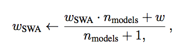
where n_models is the number of models already included in the average, w_swarepresents the weights of the copy, and w represents the weights of the model being trained. This amounts to storing the running average of the models seen at the end of each epoch of training.
And that’s the meat of the algorithm! But the paper introduces a few additional wrinkes. First, the authors develop specific learning rate schedules to ensure that SGD is exploring good optima when you start to average the models.
Additionally, you generally want to pre-train the network for a certain amount of epochs to start, as opposed to starting to track the average from the beginning . Also, if you’re using cyclical learning rates, you want to store the average at the end of each cycle, rather than after each epoch.
Finding Wider Optima
As an explanation for how SWA works, the authors provide evidence that it causes the model to end up at a wider local optimum than just SGD would. Finding a wider optimum can improve the ability of a model to generalize, because the loss surfaces of the train and test data might not be exactly aligned. Thus, being in a wider optimum for the training data makes it more likely that the model is also at an optimum for the test data.
This can be seen in one of the diagrams from the paper, here:
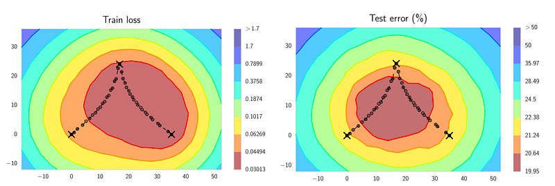
You can see how the training loss (left) and the test error (right) are similar, but not exactly the same. For example, the rightmost X is at an optimal point in the training loss surface, but is some distance away from the optimal test error. It is these differences that make it better to find a wider optimum, one that is more likely to be in a good spot for both train and test loss.
So does SWA actually lead to the discovery of wider optima? The authors provide experimental evidence to support that idea. In Section 3.4 of their paper, called Optima Width, they propose the following: in order to compare the width of the optima that are discovered by SGD and SWA, you can measure the loss as a function of the distance from the optima in a given direction. The authors sampled 10 different directions and measured the loss for a Preactivation Resnet trained on CIFAR-10 with SGD and SWA, and the results were:
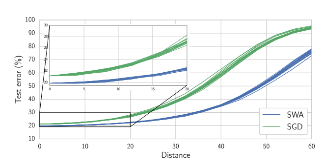
The figure provides evidence that the optima found by SWA is wider than the one found by SGD, since it takes a greater distance from the SWA optimum to increase the test error by the same amount. For example, to get to a test error of 50% you’d have to travel a distance of about 30 from the SGD optimum, compared to about 50 for SGD.
Experiments
The authors performed a number of experiments to validate the SWA method on different datasets and model architectures. To start, I’ll describe in detail the setup of the experiments that I tried to replicate during my implementation of the algorithm, and then I’ll go over some of the other key results.
The experiments that I chose for replication were done on CIFAR-10, using the VGG16 and Preactivation-Resnet-110 architectures (the authors also included Wide ResNet28–10 and Shake-Shake2x64d in their paper). For each architecture, a certain budget was chosen, to represent the number of epochs needed to train the model to convergence using just SGD+momentum. For VGG the budget was 200, while for Resnet it was 150. The models were trained with SGD+momentum for a single budget. Then, to test SWA, the models were trained with SGD+momentum for about 75% of the budget, and then trained with SWA for additional epochs to reach 1, 1.25, and 1.5 times the original budget. For each tests, three models were trained, and the mean and standard deviation were reported.
In addition to the experiments on CIFAR-10, the authors performed similar experiments on CIFAR-100. They also tested pretrained models on ImageNet, running for an additional 10 epochs with SWA, and found improved accuracies on pretrained ResNet-50, ResNet152, and DenseNet-161. Finally, the authors showed success training a Wide ResNet-28–10 from scratch using SWA with a fixed learning rate.
For further detail, you can find the paper, “Averaging Weights Leads to Wider Optima and Better Generalization”, here.
Implementation
Having read through the paper a few times and digested it, I jumped into the fast.ai library to figure out where I should actually add the code to get SWA working.
Since the fast.ai library provides the ability to add custom callbacks, I decided that that was the right place to implement the algorithm. If I wrote a callback with a hook that was called at the end of each epoch, I would be able to update the running average of the weights at the appropriate time. This is the code I ended up with:
The callback takes three parameters: model, swa_model, and swa_start. The first two are just the model we’re training, and the copy of the model that we will use to store the average of the weights once SWA begins. The swa_start parameter is the epoch when the averaging begins, since in the paper the model is always trained for a certain number of epochs with SGD+momentum before starting to track the average weights.
From there, you can see how the SWA callback translates the algorithm from the paper into Pytorch code. If we reach the epoch where SWA begins, we update the running average of the parameters, and then increment our count of the number of models included in the average (called swa_n).
Beyond the code for the callback that would perform the bulk of the algorithm, I also needed to include code to fix the running averages of batchnorm before the SWA model could do inference. As the authors explain in the paper, “If the DNN uses batch normalization [Ioffe and Szegedy, 2015], we need to compute the running mean and standard deviation of the activations for each layer of the network found by SWA after the training is finished.” The batchnorm layer normally computes these running statistics during training, but since the model’s weights are computed as the average of other models, these running stats will be wrong for the activations of the SWA model, so another single pass through the data is required to let the batchnorm layers calculate the correct running statistics.
The code for the fix looks like this:
Finally, there was the matter of making sure that the code I wrote for SWA was placed in the correct spot in the training loop. This required me to learn more about how the fast.ai library actually runs through the epochs to fit the model. I had to make some modifications to the fit method of learner.py, and additionally added some code to model.py to run validation using the SWA model in additional to the model being trained.
For a full view of the changes that were necessary to get this working in fast.ai, you can see the diff from my pull request here.
Testing
Coming from a background in software engineering, testing is something that I place a lot of importance on. But it can be hard to apply something like unit testing to machine learning code, either because of some non-deterministic elements in your training, or because of the time it would take to get to the state you actually want to test. (Check out this blog post—How to unit test machine learning code.—for a longer discussion of using unit testing in machine learning.)
Even if I couldn’t apply true unit testing to the code I was writing, I still wanted some way to make sure what I was doing was actually working (and that I wasn’t breaking other parts of the library in the process). In order to do that, I made two “test” notebook—one, the “functional” tests, were smaller chunks of code, often running on simpler models, that were meant to answer the question, “Does this function do what I think it does?”. For example, one functional test checked that, after several epochs of training, the SWA model actually equaled the average of the parameters of all the SGD models:
These tests, which could typically run in under 30 seconds, were a big help as I wrote the implementation, to alert me when things were broken. Since the pace of development on the fast.ai library is currently very fast, these tests also helped me quickly identify problems when trying to resolve merge conflicts with the master branch.
The second test notebook I made was for what I called “experimental” tests. It was meant to answer the question, “If I try to recreate the paper’s experiments using my implementation and the fast.ai library, do I observe the same results as the paper?” I ran these tests once I had a functional implementation, to determine whether SWA would make a useful contribution to the library. These experiments took much longer than the functional tests (roughly 3–4 hours for each PreResNet110 model on my 1080ti, for 12 models), but were a good final check that everything was working as expected.
In the end I was able to replicate the results of the paper—Stochastic Weight Averaging does produce higher accuracy on CIFAR-10 than normal SGD with momentum, and the improvement generally increases along with the number of training epochs. As you can see in the tables below, all of my results had better accuracy than those from the original paper, which is something that I’m still investigating. One factor might be the way data augmentations are done—for CIFAR-10 the augmentations include padding each image by 4 pixels and taking a random crop, and I found that fast.ai uses a different kind of padding (reflection padding) by default. The pattern of improvement of SWA over SGD+momentum, however, can be clearly seen.
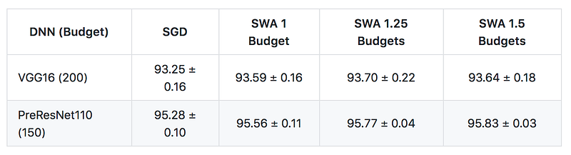
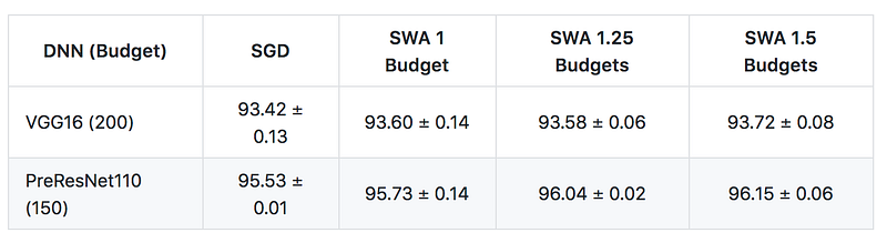
(The code I wrote for testing can be found in this gist.)
Conclusion
I was very happy with the end results of this project, as I was able to replicate an experiment from a cutting-edge research paper and make my first contribution to a machine learning open source project. I owe a big thanks, first of all, to Jeremy and Rachel from fast.ai—I have learned so much from you, and I’m grateful to have discovered the course and to have the chance to be an International Fellow this time around. Also, thank you to the researchers, Pavel Izmailov, Dmitrii Podoprikhin, Timur Garipov, Dmitry Vetrov, Andrew Gordon Wilson, who wrote this great paper.
And now I’d like to encourage everyone to download the fastai library and give SWA a try! I’m particularly interested to see people start applying it to their own image datasets (beyond CIFAR and Imagenet), as well as exploring the possibility of using it outside of the domain of computer vision.


