AdaBoost Illustrated

AdaBoost (short for Adaptive Boosting) is a powerful boosting algorithm that can boost the performance of any machine learning model. It was introduced in 1995 by Freund and Shapira [1], who won the 2003 Gödel Prize (one of the most prestigious prizes in Computer Science) for their work. It is still one of the most popular boosting algorithms used today.

This article explains the AdaBoost algorithm in detail, demonstrates its usage on a toy example, and shows you how to run it using Scikit-Learn.

Background: Boosting Methods

Boosting is an ensemble method (see this article for an introduction on ensemble methods), where the base models are trained in sequence. Each model focuses on correcting the errors made by the previous models.

In AdaBoost, samples that are misclassified by one model are assigned greater weight when used to train the next model. Each model is thereby forced to concentrate on examples that were misclassified by the previous ones.

The predictions of the models are then combined using a weighted majority vote, where the weights are based on how well each model performed on the training set.

The base learners used in boosting are usually weak learners, i.e., models whose accuracy is only slightly better than a random guesser (50% + ϵ, for a small ϵ). The advantage of weak learners is that they are fast to train and they suffer less from overfitting.

A weak learner that is often used is a decision stump. A decision stump is a decision tree with only one level, i.e., a tree with only one split:

The AdaBoost Algorithm

The algorithm takes as input a training set {(x₁, y₁), (x₂, y₂), … , (xₙ, yₙ)}, where each xᵢ belongs to some input space X (typically xᵢ is a vector), and yᵢ is a binary label that takes the values 1 or -1.

The algorithm itself consists of T boosting rounds. In each round t (t = 1, …, T), we train a weak classifier using a weak or a base learning algorithm (e.g., a decision stump learner).

In addition, the algorithm maintains a distribution or set of weights over the training set, denoted by D. The weight of this distribution on training sample i in round t is denoted by Dₜ(i).

Initially, the weights of all the samples are equal, i.e., in round 1 we have:

In each successive round, the weights of misclassified samples are increased so that the weak learner is forced to focus on the hard samples in the training set.

The weak learner’s objective if to find a weak hypothesis X → {-1, +1} appropriate for the distribution Dₜ. In practice, the weak learner may be a learning algorithm that can use the weights Dₜ on the training samples directly. Alternatively, a set of the training examples can be sampled according to Dₜ, and these (unweighted) resampled examples can be used to train the weak learner.

The quality of the weak hypothesis is measured by its error rate ϵ, defined as its probability of misclassifying a training example:

Note that the error is measured with respect to the distribution Dₜ on which the weak learner was trained.

The weak learner is then assigned an importance factor α that determines its contribution to the ensemble’s overall prediction, and depends on its error rate:

η (eta) is a learning rate hyperparameter, typically set to 0.5. Note that αₜ > 0 when ϵₜ < 0.5 (which should be true since the model is a weak learner), and that αₜ gets larger as ϵₜ gets smaller (i.e., a more successful learner contributes more to the ensemble’s prediction).

Then, the distribution Dₜ is updated according to the following rule:

where Zₜ is a normalization factor that makes sure that D remains a distribution in the next round:

The effect of this rule is to increase the weight of the samples misclassified by hₜ, and to decrease the weights of correctly classified samples. This is because for a misclassified sample we have yᵢ ≠ hₜ(xᵢ). Since both yᵢ and hₜ(xᵢ) are either 1 or -1, this means that yᵢhₜ(xᵢ) = -1. Therefore, the update rule for this sample becomes:

The last inequality derives from the fact that αₜ > 0, thus exp(αₜ) > 1.

Similarly, for a correctly classified sample, we have yᵢ = hₜ(xᵢ), hence yᵢhₜ(xᵢ) = -1, and the update rule for this sample is:

The final hypothesis H of the ensemble is a weighted majority vote of the T weak hypotheses, where αₜ is the weight assigned to hₜ:

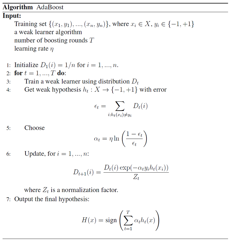
The following pseudocode shows the entire algorithm:

Toy Example

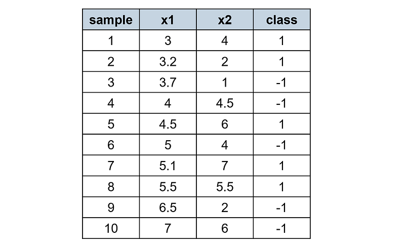
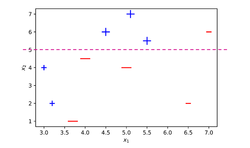
Assume that we have the following training set with 10 two-dimensional examples:

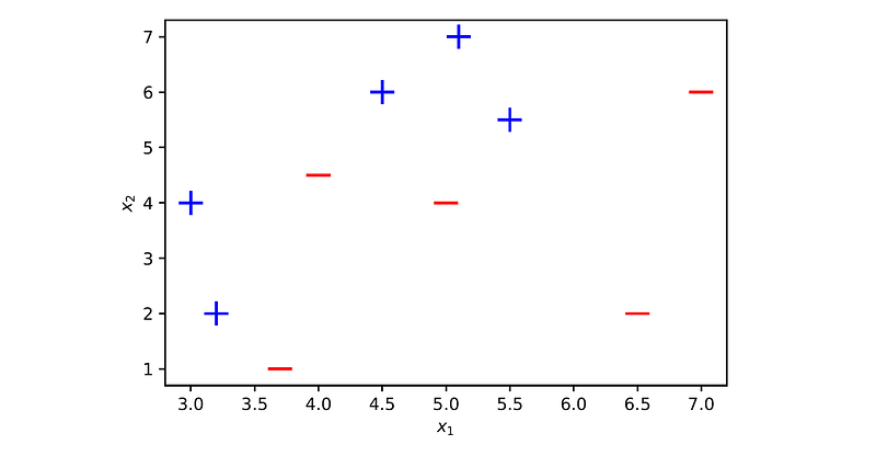
Let’s plot these examples:

Next, we will run three rounds of boosting on this training set.

First Boosting Round

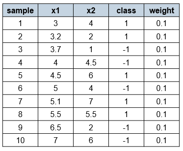
In the first round, the weights of all the examples are equal to 0.1:

We now try to fit our first decision stump to these examples. A decision stump can use only one of the features x₁ or x₂ to make a decision. Since all the examples have an equal chance to get selected, the best decision stump we can get in the first round is x₁ ≤ 3.5, where the left class is 1 and the right class is -1.

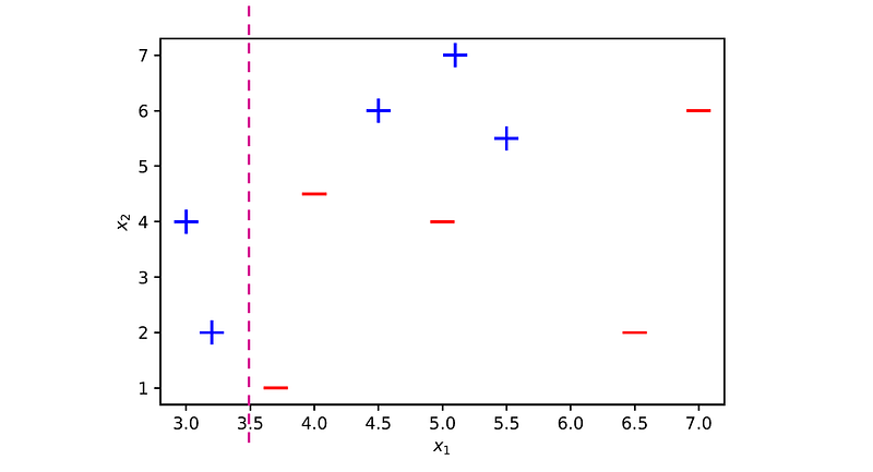
This stump has only three errors: it misclassifies samples 5, 7, and 8. Therefore, its error rate is ϵ₁ = 3 ⋅ 0.1 = 0.3, and its importance factor is:

We now compute the new distribution of the samples. The new weight of the misclassified samples 5, 7, and 8 (before normalization) is:

i.e., the weights of the misclassified samples increased from 0.1 to 0.153.

And the new weight of the correctly classified samples (before normalization) is:

i.e., the weights of the correctly classified samples decreased from 0.1 to 0.065.

The normalization factor is just the sum of all the new weights:

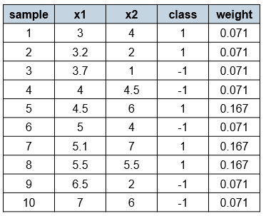
Therefore, the new weights after normalization are:

So the distribution of the samples before the second boosting round is:

Second Boosting Round

In the second round, samples 5, 7, and 8 that were misclassified have a higher chance to be selected. Therefore, the second decision stump will give a higher priority to classifying these samples correctly. Such a decision stump could be for example, x₁ ≤ 6, where the left class is 1 and the right class is -1.

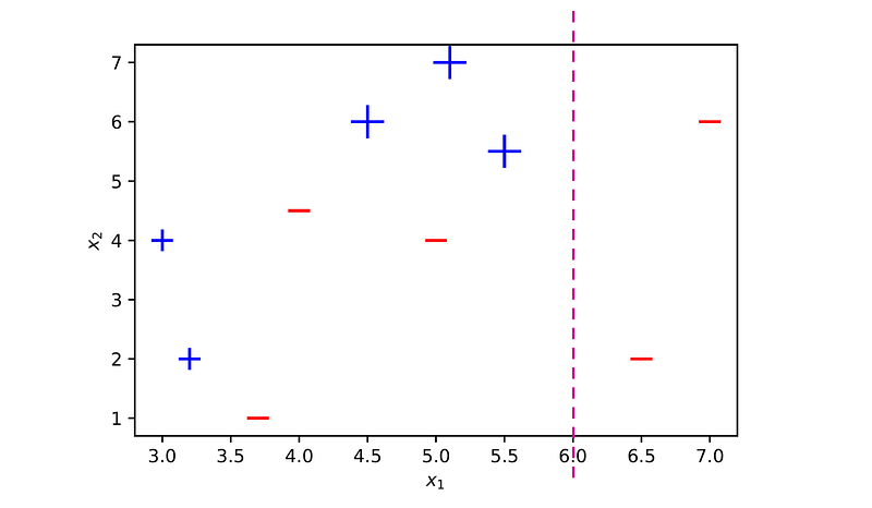
This learner misclassifies only three samples (3, 4 and 6), all of which have lower weights. Therefore, its error rate is ϵ₂ = 3 ⋅ 0.071 = 0.213, and its importance factor is:

The new distribution of the weights (after normalization) is:

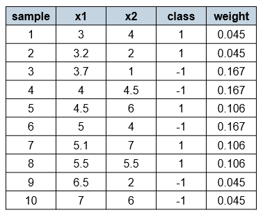
Third Boosting Round

The third decision stump will give the highest priority to samples 3, 4 and 6, that were misclassified in the second round, and the second-highest priority to samples 5, 7 and 8 that were misclassified in the first round. A decision stump that classifies all these six samples correctly is x₂ ≥ 5.

This decision stump misclassifies samples 1, 2, and 10. Therefore, its error rate is ϵ₃ = 3 ⋅ 0.045 = 0.135, and its importance factor is:

The Final Hypothesis

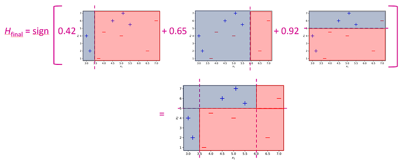
The final hypothesis consists of a weighted average of the three decision stumps:

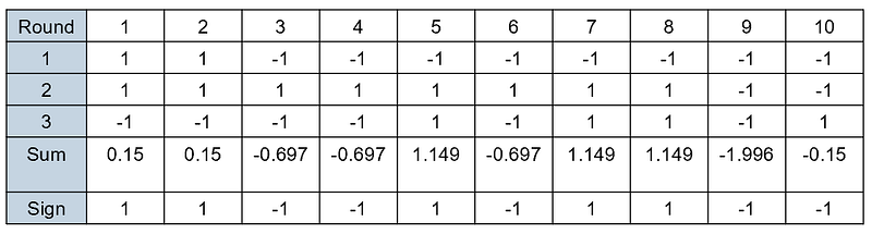
As we can see in the last row of the table, the final ensemble classifies all the training samples perfectly!

Visually, the final ensemble looks as follows:

Analyzing the Training Error

An important theoretical property of AdaBoost is that the training error of the ensemble decreases exponentially as a function of the number of boosting rounds.

Let us write the error ϵₜ of hₜ as 0.5-γₜ. Since a random guesser has an error rate of 0.5, γₜ measures how much better are the predictions of weak learner t than random.

Freund and Schapire [1] have shown that the training error of the final hypothesis H is at most

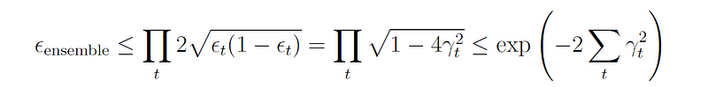
If each weak learner is slightly better than random, we can write γₜ ≥ γ for some γ > 0, thus we get:

In other words, the ensemble’s error on the training set drops exponentially fast in T (the number of rounds).

The meaning of this result is that AdaBoost can efficiently transform any weak learning algorithm into a strong learning algorithm.

AdaBoost in Scikit-Learn

Scikit-Learn provides two classes that implement the AdaBoost algorithm:

1. AdaBoostClassifier is used for classification problems. It is based on an algorithm called AdaBoost-SAMME [2], which is an extension of AdaBoost to multi-class problems.
2. AdaBoostRegressor is used for regression problems. It is based on an algorithm known as AdaBoost.R2 [3], which extends AdaBoost to regression problems.

The important parameters of these classes are:

• base_estimator — the base estimator from which the ensemble is built. By default, the base estimator is a DecisionTreeClassifier with max_depth=1 (i.e., a decision stump).
• n_estimators — the number of base estimators to train (defaults to 50).
• learning_rate — the weight applied to each estimator, which controls its contribution to the final prediction (defaults to 1.0).

For example, let’s train an AdaBoost classifier on the Iris data set, using only the first two features of each flower (sepal width and sepal length). In the previous article on decision trees, we have seen that a fully-grown tree can achieve on this data set a test accuracy of 65.79%, while a pruned decision tree (with max_depth = 3) obtained a test accuracy of 76.32%. Let’s see if we can do better with AdaBoost.

First, we fetch the data:

from sklearn.datasets import load_iris

iris = load_iris()
X = iris.data[:, :2] # we only take the first two features
y = iris.target

Then we split it into training and test sets:

from sklearn.model_selection import train_test_split

X_train, X_test, y_train, y_test = train_test_split(X, y, random_state=42)

Next, we instantiate an AdaBoostClassifier with its default settings (i.e., an ensemble of 50 decision stumps) and fit it to the training set:

from sklearn.ensemble import AdaBoostClassifier

clf = AdaBoostClassifier(random_state=42)
clf.fit(X_train, y_train)

Similar to a DecisionTreeClassifier, we fix the random state of the AdaBoostClassifier in order to allow reproducibility of the results.

Let’s check the model’s performance on both the training and test sets:

print(f'Train accuracy: {clf.score(X_train, y_train):.4f}')
print(f'Test accuracy: {clf.score(X_test, y_test):.4f}')

Train accuracy: 0.7143
Test accuracy: 0.7368

The model performs better than the fully-grown decision tree but worse than the pruned tree.

Let’s plot the decision boundaries of the model:

from matplotlib.colors import ListedColormap

def plot_decision_boundaries(clf, X, y, feature_names, class_names, 
                             colors=['r', 'b'], markers=('s', 'o')):  
    cmap = ListedColormap(colors)
      
    # Create a mesh of n sample points in the range [x1_min, x1_max] x [x2_min, x2_max]
    n = 1000 
    x1_min, x1_max = X[:, 0].min() - 1, X[:, 0].max() + 1
    x2_min, x2_max = X[:, 1].min() - 1, X[:, 1].max() + 1 
    x1, x2 = np.meshgrid(np.linspace(x1_min, x1_max, n), np.linspace(x2_min, x2_max, n))
    
    # Find the label of each point in the mesh
    y_pred = clf.predict(np.c_[x1.ravel(), x2.ravel()])
    y_pred = y_pred.reshape(x1.shape) 
    
    # Put the result into a color plot  
    plt.contourf(x1, x2, y_pred, cmap=cmap, alpha=0.4)
    
    # Plot the points from the data set
    sns.scatterplot(x=X[:, 0], y=X[:, 1], hue=class_names[y], style=class_names[y], 
                    palette=colors, markers=markers, edgecolor='k')
    
    plt.xlabel(feature_names[0])
    plt.ylabel(feature_names[1])
    plt.legend()

plot_decision_boundaries(clf, X, y, iris.feature_names, iris.target_names)

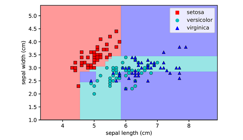
Note that the decision boundaries of AdaBoost are rectilinear, since the final ensemble consists of a mixture of decision stumps (each of which has a linear decision boundary).

Tuning the Hyperparameters

The main hyperparameters to tune in AdaBoost are the number of estimators, its learning rate, and the complexity of the base estimators (e.g., the maximum depth of the tree or the minimum number of samples in leaf nodes).

There is a tradeoff between the number of estimators and the learning rate parameters. Decreasing the learning rate leads to smaller changes in the weight distributions D(i), which in turn reduces overfitting of the learners to noisy samples. On the other hand, it also entails more boosting rounds in order to correct the errors of the previous learners, which in turn increases the number of estimators in the ensemble and thereby makes the final model more complex and susceptible to overfitting.

For example, let’s tune the hyperparameters of the previous AdaBoostClassifier by running the following randomized search:

from sklearn.model_selection import RandomizedSearchCV
from sklearn.tree import DecisionTreeClassifier

params = {
    'base_estimator__max_depth': np.arange(1, 11),
    'n_estimators': [10, 50, 100, 200, 500],
    'learning_rate': np.arange(0.1, 1.0, 0.1),
}

base_estimator = DecisionTreeClassifier(random_state=42)
search = RandomizedSearchCV(AdaBoostClassifier(base_estimator, random_state=42), params, 
                            n_iter=50, cv=3, n_jobs=-1)
search.fit(X_train, y_train)

print(search.best_params_)

Note that in order to tune the parameters of the decision tree that is used as a base estimator, you need to define it explicitly and pass it to the constructor of AdaBoostClassifier. Then, in the search parameters you can use the prefix ‘base_estimator__[decision tree parameter]’ to refer to the parameters of the decision tree.

The best model found by the search is:

{'n_estimators': 10, 'learning_rate': 0.7000000000000001, 'base_estimator__max_depth': 8}

And its performance on the training and test sets is:

best_clf = search.best_estimator_
print(f'Train accuracy: {best_clf.score(X_train, y_train):.4f}')
print(f'Test accuracy: {best_clf.score(X_test, y_test):.4f}')

Train accuracy: 0.9554
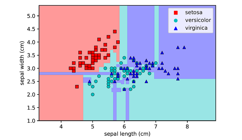
Test accuracy: 0.7368

The accuracy on the training set has improved significantly (from 71.43% to 95.54%), while the accuracy on the test set has remained the same. This suggests that the model overfits to the outliers in the training set, as confirmed by examining its decision boundaries:

Summary

Let’s summarize the pros and cons of AdaBoost as compared to other supervised machine learning models:

Pros:

• Can provide highly accurate models, as each weak learner improves the areas where previous models performed poorly.
• Has strong theoretical guarantees regarding the training error (the error decreases exponentially in the number of boosting rounds).
• Less prone to overfitting, since it is built from an ensemble of weak learners, where each learner underfits the training set.
• Can handle various types of data, including numerical and categorical features.
• Provides a measure of feature importance.
• Can be applied to both classification and regression tasks.

Cons:

• Sensitive to outliers and mislabeled data points, since examples that are difficult to classify are assigned ever-increasing weights in successive boosting rounds.
• Training can be computationally intensive when dealing with large data sets or when the number of weak models is large. In addition, the training cannot be parallelized (unlike in random forests for example).
• Relies on the performance of the weak models. If these are too complex or biased, it may lead to poor results.
• Less interpretable than simpler models, such as decision trees or linear regression.
• Has several hyperparameters that need to be tuned, such as the number of boosting iterations and the learning rate.
• Prediction can be slower compared to other models, as it requires traversing multiple trees and aggregating their predictions.

Final Notes

You can find the code examples of this article on my github: https://github.com/roiyeho/medium/tree/main/adaboost

Thanks for reading!

References

[1] Yoav Freund and Robert E. Schapire. A decision-theoretic generalization of on-line learning and an application to boosting. Journal of Computer and System Sciences, 55(1):119–139, 1997.

[2] Zhu, H. Zou, S. Rosset, T. Hastie. Multi-class AdaBoost. Statistics and its Interface, 2(3):349–360, 2009.

[3] Harris Drucker. Improving Regressors using Boosting Techniques. Icml, vol. 97, pp. 107–115, 1997.