
Actual vs Predicted: Evaluating Stock Price Predictions
Analyzing the Performance of a Machine Learning Model in Stock Forecasting
Predicting stock prices is a challenging yet crucial task for investors and financial analysts. In this analysis, we delve into the performance of a Long Short-Term Memory (LSTM) neural network model designed to forecast stock prices. The model is trained on historical stock data, aiming to capture the underlying patterns and trends to make accurate future predictions. We evaluate the model’s effectiveness by comparing its predictions on test data against the actual stock prices, highlighting the precision and potential areas for improvement. Through visual representation, we aim to provide a clear and concise comparison, enabling a better understanding of the model’s predictive capabilities in the dynamic and unpredictable realm of the stock market.
This step involves bringing in the necessary packages for use in the program.
Importing essential libraries for data analysis, visualization, and deep learning
import math # Mathematical functions
import numpy as np # Fundamental package for scientific computing with Python
import pandas as pd # Additional functions for analysing and manipulating data
import matplotlib.dates as mdates # Formatting dates
import matplotlib.pyplot as plt # Important package for visualization - we use this to plot the market data
import tensorflow as tf
from sklearn.metrics import mean_absolute_error, mean_squared_error # Packages for measuring model performance / errors
from tensorflow.keras import Sequential # Deep learning library, used for neural networks
from tensorflow.keras.optimizers import Adam
from tensorflow.keras.layers import LSTM, Dense, Dropout,Activation # Deep learning classes for recurrent and regular densely-connected layers
from tensorflow.keras.callbacks import EarlyStopping # EarlyStopping during model training
from sklearn.preprocessing import MinMaxScaler # This Scaler removes the median and scales the data according to the quantile range to normalize the price data
import seaborn as sns # Visualization
import plotly.graph_objects as go
This code imports Python libraries commonly used for mathematical and scientific calculations, data analysis, visualization, and deep learning. Each library has a specific purpose to fulfill these tasks effectively. The math module provides functions for common mathematical operations, such as square roots and logarithms. numpy is a key tool for scientific computing in Python. It allows users to work with extensive multi-dimensional arrays and matrices, as well as provides essential mathematical functions that can be performed on these arrays. Pandas is a library in Python that offers added features to help with analyzing and working with data, particularly when it is structured in tables. Matplotlib is a Python library that enables users to create various types of visualizations, such as static, animated, and interactive plots. In the context of market data, matplotlib is commonly utilized for plotting data and adjusting date formats on the plots. Tensorflow is a library used for deep learning. It helps in creating and training neural networks. Sklearn is a set of tools that are used for machine learning and statistical modeling. It includes various metrics that help in evaluating the performance of models. Seaborn is a data visualization library built on top of matplotlib. It offers a simple way to generate visually appealing and informative statistical graphics. Plotly is a tool for creating interactive visualizations like plots, charts, and graphs with various interactive features. This code prepares the software environment for conducting data analysis, visualization, and deep learning tasks by importing the required libraries and modules.
This section involves bringing in information.
Reading and preprocessing a CSV file into a pandas DataFrame.
def read_df(csv_file):
    df = pd.read_csv(csv_file)
    df["Date"]=pd.to_datetime(df["Date"])
    df.index=df["Date"]
    df.drop("Date",axis=1,inplace=True)
    return df
csv_file = "data\\NABIL_LARGE.csv"
df = read_df(csv_file)
This code converts a CSV file into a pandas dataframe. It converts the “Date” column to a datetime format and makes it the index. Then the code removes the “Date” column and returns the updated dataframe. You will be using the “NABIL_LARGE.csv” file, which is stored in the data folder.
DataFrame containing the data from the CSV file
df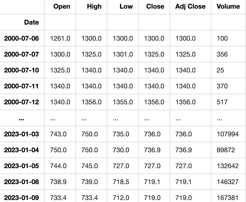
In Python, the variable name “df” is commonly used to refer to a DataFrame object, especially within libraries like Pandas. A DataFrame is a structured way to store data in rows and columns, often used for data analysis and manipulation. The “df” variable holds this data and can be modified, analyzed, and displayed visually for further insights.
Here we will analyze and investigate the data to gain insights and understanding.
Plotting the data from the DataFrame
def plot_data(df):
    df_plot = df.copy()
    print(df_plot.shape)
    ncols = 2
    nrows = int(round(df_plot.shape[1] / ncols, 0))

    fig, ax = plt.subplots(nrows=nrows, ncols=ncols, sharex=True, figsize=(14, 7))
    for i, ax in enumerate(fig.axes):
            sns.lineplot(data = df_plot.iloc[:, i], ax=ax)
            ax.tick_params(axis="x", rotation=30, labelsize=10, length=0)
            ax.xaxis.set_major_locator(mdates.AutoDateLocator())
    fig.tight_layout()
plt.show(plot_data(df)) (4928, 6)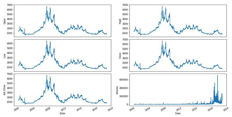
This code creates a function named ‘plot_data’ that takes a DataFrame as its input. The function makes a copy of the DataFrame and calculates the number of rows and columns needed for the plot based on the DataFrame’s shape. It then uses Matplotlib to generate a subplot figure with the defined number of rows and columns. The function generates a line plot for each subplot using Seaborn’s ‘lineplot’ function, with the data from the respective column of the DataFrame. It further adjusts the x-axis ticks by rotating them, resizing labels, and setting the major tick locator. The function organizes the subplots neatly by using ‘tight_layout’ and then shows the plot using Matplotlib’s ‘show’ function. Before running this code, make sure you have imported the required libraries like pandas, matplotlib, seaborn, and matplotlib.dates.
Feature engineering is a process in machine learning where we create new input features from existing ones to help improve the performance of a model. It involves transforming, selecting, or combining features to make them more suitable for the algorithm being used. This step is crucial for building efficient and accurate machine learning models.
Creating features from the given data and returning a DataFrame
def createFeatures(data):
    data = pd.DataFrame(data)


    data['Close_Diff'] = data['Adj Close'].diff()

    data['MA200'] = data['Close'].rolling(window=200).mean()
    data['MA100'] = data['Close'].rolling(window=100).mean()
    data['MA50'] = data['Close'].rolling(window=50).mean()
    data['MA26'] = data['Close'].rolling(window=26).mean()
    data['MA20'] = data['Close'].rolling(window=20).mean()
    data['MA12'] = data['Close'].rolling(window=12).mean()

    data['DIFF-MA200-MA50'] = data['MA200'] - data['MA50']
    data['DIFF-MA200-MA100'] = data['MA200'] - data['MA100']
    data['DIFF-MA200-CLOSE'] = data['MA200'] - data['Close']
    data['DIFF-MA100-CLOSE'] = data['MA100'] - data['Close']
    data['DIFF-MA50-CLOSE'] = data['MA50'] - data['Close']

    data['MA200_low'] = data['Low'].rolling(window=200).min()
    data['MA14_low'] = data['Low'].rolling(window=14).min()
    data['MA200_high'] = data['High'].rolling(window=200).max()
    data['MA14_high'] = data['High'].rolling(window=14).max()
    data['MA20dSTD'] = data['Close'].rolling(window=20).std()

    data['EMA12'] = data['Close'].ewm(span=12, adjust=False).mean()
    data['EMA20'] = data['Close'].ewm(span=20, adjust=False).mean()
    data['EMA26'] = data['Close'].ewm(span=26, adjust=False).mean()
    data['EMA100'] = data['Close'].ewm(span=100, adjust=False).mean()
    data['EMA200'] = data['Close'].ewm(span=200, adjust=False).mean()

    data['close_shift-1'] = data.shift(-1)['Close']
    data['close_shift-2'] = data.shift(-2)['Close']

    data['Bollinger_Upper'] = data['MA20'] + (data['MA20dSTD'] * 2)
    data['Bollinger_Lower'] = data['MA20'] - (data['MA20dSTD'] * 2)

    data['K-ratio'] = 100*((data['Close'] - data['MA14_low']) / (data['MA14_high'] - data['MA14_low']) )
    data['RSI'] = data['K-ratio'].rolling(window=3).mean()

    data['MACD'] = data['EMA12'] - data['EMA26']

    nareplace = data.at[data.index.max(), 'Close']
    data.fillna((nareplace), inplace=True)

    return data
The code introduces a function named createFeatures that enhances a DataFrame by calculating and appending new columns (features) based on existing data. This code summary explains the functionality of the code. To calculate the daily closing price difference, a new column called Close_Diff is added. Moving averages, or MAs, are calculated for several time periods (200-day, 100-day, 50-day, 26-day, 20-day, and 12-day) and then added as new columns to the data. This function determines the variances between different moving averages and the closing price. It then includes these variances as additional columns in the data. This action computes the smallest and largest values for both low and high prices across various time frames, and then includes these values as new columns in the data. To determine the volatility of the closing price over a 20-day period, the standard deviation is calculated. This value is then added to the data table as a new column. The tool computes exponential moving averages (EMA) for various time periods and includes them as additional columns. Two new columns are added by shifting the closing price by 1 and 2 days, creating lagged versions of the data. The upper and lower Bollinger Bands are determined by using the 20-day moving average and standard deviation. The K-ratio and Relative Strength Index (RSI) are calculated using the lowest and highest prices observed over a 14-day period. The Moving Average Convergence Divergence (MACD) is a technical indicator that is calculated by subtracting the 26-day Exponential Moving Average (EMA) from the 12-day EMA. This action involves replacing any empty cells in the dataset with the most recent closing price available. The function ultimately returns the DataFrame with the new features included.
DataFrame with added features
df = createFeatures(df)
df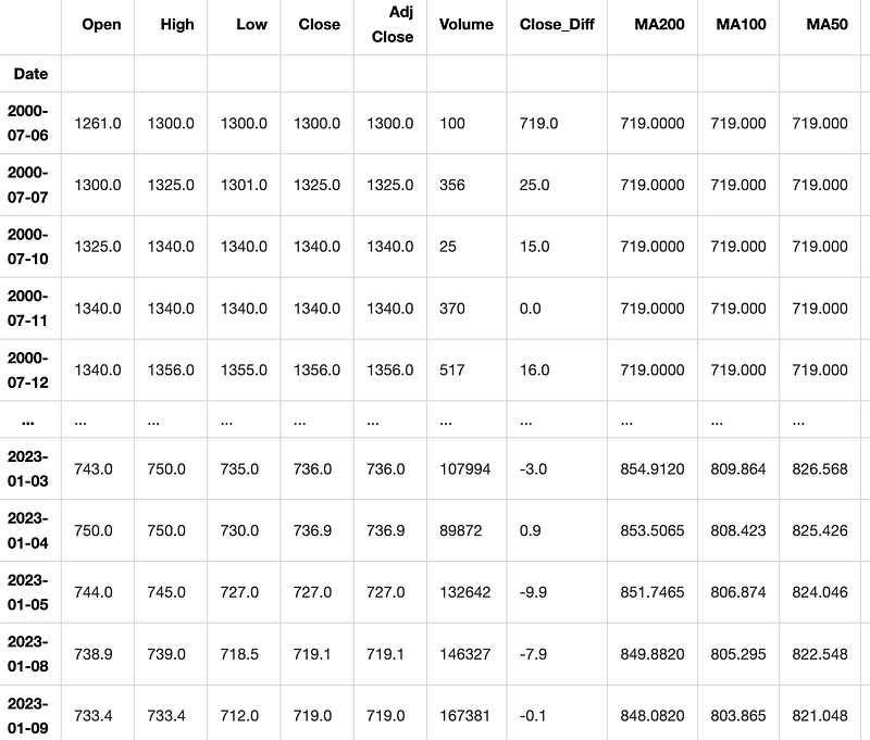
This code uses a function called “createFeatures” to modify a DataFrame named “df” by adding new columns. The function takes “df” as input and after it runs, the updated DataFrame with the new columns is printed out.
Preprocessing and feature selection are important steps in preparing data for machine learning models. Preprocessing involves cleaning, scaling, and transforming the data to make it suitable for analysis. Feature selection is the process of choosing the most relevant features in the dataset that will contribute to the predictive power of the model. These steps help improve the accuracy and efficiency of machine learning algorithms by reducing noise and redundant information in the data.
Filtering data to include only selected features
def filter_data(df):

    train_df = df.sort_values(by=['Date']).copy()

    FEATURES = ['Volume', 'High', 'Low', 'Open', 'Bollinger_Upper', 'Bollinger_Lower', 'Close'#,'RSI', 'MACD',
               ]

    print('FEATURE LIST')
    print([f for f in FEATURES])

    data = pd.DataFrame(train_df)
    data_filtered = data[FEATURES]
    return data_filtered
data_filtered = filter_data(df)
data_filtered
FEATURE LIST
['Volume', 'High', 'Low', 'Open', 'Bollinger_Upper', 'Bollinger_Lower', 'Close']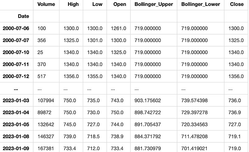
This code creates a function named filter_data which operates on a DataFrame. It begins by sorting the input DataFrame based on the ‘Date’ column, making a copy of the sorted DataFrame. It then defines a list of features called FEATURES and prints this list. Next, it converts the sorted DataFrame into a new pandas DataFrame named ‘data’. Finally, it filters the ‘data’ DataFrame to include only the columns listed in the FEATURES list and returns this filtered DataFrame. To successfully run the code, make sure to import the pandas library at the start of your script.
Correlation of each feature with the ‘Close’ price
data_filtered.corr()['Close']Volume -0.167459
High 0.999675
Low 0.999522
Open 0.998140
Bollinger_Upper 0.972728
Bollinger_Lower 0.983736
Close 1.000000
Name: Close, dtype: float64This code computes the correlation coefficient between the ‘Close’ column and all other columns in the ‘data_filtered’ dataset. The correlation coefficient shows how the ‘Close’ column is related to each of the other columns, with a value that can range from -1 to 1. A value close to 1 indicates a strong positive relationship between the variables. When the value is close to -1, it indicates a strong negative relationship between the variables. When a value is close to 0, it indicates that there is either no relationship or a very weak relationship between the variables being studied. This code helps determine the degree of correlation between the ‘Close’ column and the other columns in the dataset. Understanding this relationship is crucial for predictions and data analysis.
Train test split is a common technique used in machine learning to divide a dataset into two subsets: one for training the model and one for testing the model. This allows us to train the model on one portion of the data and then evaluate its performance on previously unseen data. Typically, the training subset is larger, aiding in better model training, while the testing subset helps to measure the model’s accuracy and generalization capabilities.
Splitting the dataset into train and test sets
def train_test_split(df):
    sequence_length = 100
    split_index = math.ceil(len(df) * 0.7)
    train_df = df.iloc[0:split_index, :]
    test_df = df.iloc[split_index - sequence_length:, :]
    return train_df, test_df,split_index
The code creates a function named train_test_split that uses a dataframe as its argument. The function divides the dataframe into a training set and a testing set. It does this by selecting a sequence length and splitting the data based on a 70-30 ratio, where 70% is allocated to the training set and 30% to the testing set. The variable sequence_length is assigned a value of 100, indicating that every sequence will have a length of 100. The code calculates the index to split the input dataframe by using the formula math.ceil(len(df) * 0.7). This index marks the location where 70% of the data will be used for training and the remaining 30% for testing.
It assigns the rows from the beginning up to the split index to the training dataframe called train_df. The code assigns rows in a dataframe, starting from a specific index minus a given sequence length and ending at the last row, to a new dataframe called test_df. At the end, it provides back the training data set, testing data set, and the split index. This code function divides a dataset into two sets - a training set and a testing set. The training set consists of the first 70% of the data, while the testing set contains the remaining 30% of the data plus some rows from the past based on a specified sequence length.
Test data after splitting
train_data, test_data, split = train_test_split(data_filtered)
test_data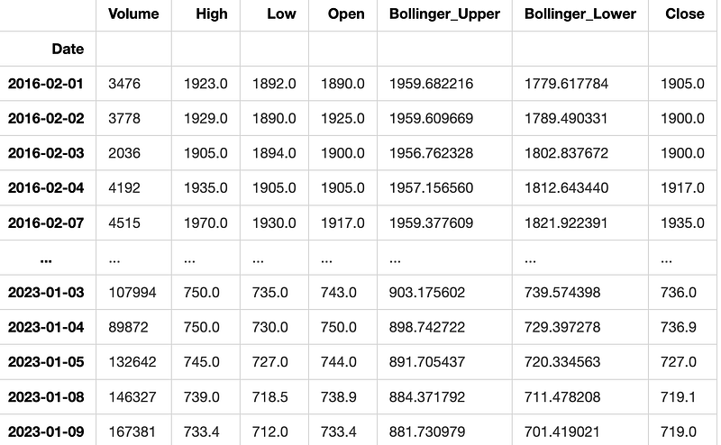
This code divides a dataset into two parts for training and testing using the train_test_split function. The training data is stored in the train_data variable, the testing data in test_data, and the ratio of the split in the split variable. Lastly, it shows the contents of the test_data variable.
Preprocessing the data by scaling it using MinMaxScaler
def preprocess_data(data):
    nrows = data.shape[0]
    np_data_unscaled = np.array(data)
    np_data = np.reshape(np_data_unscaled, (nrows, -1))
    print(np_data.shape)
    scaler = MinMaxScaler()
    np_data_scaled = scaler.fit_transform(np_data_unscaled)

    return np_data_scaled, scaler
train_data_scaled, scaler = preprocess_data(train_data)
test_data_scaled, scaler = preprocess_data(test_data)(3450, 7)
(1578, 7)The code creates a function named preprocess_data which normalizes the input data using MinMaxScaler. This code performs the following actions: Receives input data. This step involves changing the structure or format of the input data. Displays the structure of the resized data. MinMaxScaler is utilized to rescale the data. The function returns both the scaled data and the scaling method used. The code preprocesses two sets of data, train_data and test_data, by applying a function. It then stores the scaled data and scaler in variables train_data_scaled, test_data_scaled, and scaler for future use. This command will divide the dataset into two parts: x and y.
Dataset partitioning for input sequences and output values
def partition_dataset(sequence_length, data):
    x, y = [], []
    data_len = data.shape[0]
    for i in range(sequence_length, data_len):
        x.append(data[i-sequence_length:i,:]) #contains sequence_length values 0-sequence_length * columsn
        y.append(data[i,:]) #contains the prediction values for validation,  for single-step prediction

    x = np.array(x)
    y = np.array(y)
    return x, y
The code contains a function named partition_dataset, which requires two parameters to be passed: sequence_length and data. This is the reason for something to exist or be done. This function is meant to split a dataset into input sequences (x) and their corresponding output sequences (y) for training a machine learning model. The input data is typically represented as a 2D array or matrix, where each row in the array stands for a different data point. The sequence_length parameter determines the number of data points grouped together to create an input sequence. An explanation is a detailed description or clarification of a concept, idea, or process to help someone understand it better. It breaks down complex information into simpler terms. The function begins by creating two empty lists, x and y. These lists will be used to store the input and output sequences, respectively. Next, the program determines the size of the data provided by the user. It goes through the data starting from a specific index (sequence_length) all the way to the end of the data. During each iteration, a section of the data with a specific length, called sequence_length, is taken out and added to the x list. The next data point after the subsequence is extracted and added to the y list. This value is used as the prediction for that input sequence. Lastly, it changes the lists x and y into numpy arrays and then gives them back. This function organizes a dataset into groups of input sequences (x) and their corresponding output sequences (y). It is typically used to train a machine learning model.
Splitting dataset into input sequences and outputs for training and testing
sequence_length = 100
x_train, y_train = partition_dataset(sequence_length, train_data_scaled)
x_test, y_test = partition_dataset(sequence_length, test_data_scaled)
print(x_train.shape, y_train.shape)
print(x_test.shape, y_test.shape)
print(y_test)(3350, 100, 7) (3350, 7)
(1478, 100, 7) (1478, 7)
[[0.01105582 0.92376919 0.96713362 ... 0.84631807 0.90604417 0.96039604]
[0.00766166 0.92165167 0.96228448 ... 0.8466347 0.91728533 0.95764576]
[0.01392823 0.92165167 0.95743534 ... 0.84707731 0.92517898 0.94939494]
...
[0.18791488 0.04552673 0.07165948 ... 0.0764322 0.06701828 0.04015402]
[0.20731714 0.04235045 0.06707974 ... 0.07288833 0.06187189 0.03580858]
[0.237167 0.03938592 0.06357759 ... 0.07161219 0.05602654 0.03575358]]This code snippet appears to be used for a task involving machine learning or time series analysis. It is likely preparing the data for model training and testing. It does so by dividing the dataset into sequences of a predetermined length. Here is an explanation of the code’s functionality: A variable named sequence_length is assigned a value of 100. The next step involves splitting the scaled training data (train_data_scaled) into input sequences and their corresponding output sequences using the partition_dataset function. The input sequences are saved in x_train and the output sequences are saved in y_train. The partitioning process is repeated for the test data (test_data_scaled). The input sequences are stored in x_test, while the output sequences are stored in y_test. Lastly, the program will display the dimensions of the training and testing input sequences (x_train.shape, x_test.shape) and output sequences (y_train.shape, y_test.shape). The output sequences of the test data (y_test) are also displayed. The code is organizing training and testing data into input and output sequences of a specified length to prepare them for a model. It then provides information about the shapes and contents of these sequences.
Printing sequence and output
print(x_train[1][sequence_length-1][-1])
print(y_train[0][-1])
0.2238301977809937
0.2238301977809937This code snippet prints the last element of the list x_train at index 1 and position sequence_length-1, as well as the last element of the list y_train at index 0.
This step involves creating the LSTM model.
Creating LSTM model
out = y_test.shape[1]
model = Sequential()
model.add(LSTM(128, input_shape=(x_train.shape[1], x_train.shape[2]), return_sequences=True, activation='relu'))
model.add(Dropout(0.3))
model.add(LSTM(64, return_sequences=False, activation='relu'))
model.add(Dropout(0.3))
model.add(Dense(out))
optimizer = Adam(learning_rate=0.001)
model.compile(optimizer=optimizer, loss='mean_squared_error')The code initially assigns the variable ‘out’ the value equal to the number of columns present in the ‘y_test’ array. A sequential neural network model is built using the Keras library. The model is made up of two LSTM layers with 128 and 64 units each. The first LSTM layer takes input in the shape determined by the rows and columns of the x_train data. It uses ReLU activation function and outputs sequences of data. To prevent overfitting, a dropout layer is added after the first LSTM layer. This layer randomly deactivates a portion of input units by setting them to 0 during training updates. The next layer in the sequence is another Long Short Term Memory (LSTM) layer with 64 units and no return sequences. This layer is then followed by a dropout layer. To finish the process, a dense layer is included in the model. The number of output nodes in this layer aligns with the size of the output data, as represented by the ‘out’ variable. The Adam optimizer is set with a learning rate of 0.001. The model is compiled to use Adam optimizer and mean squared error as the loss function for training the neural network.
model summary
model.summary()Model: "sequential_7"
_________________________________________________________________
Layer (type) Output Shape Param #
=================================================================
lstm_14 (LSTM) (None, 100, 128) 69632
dropout_14 (Dropout) (None, 100, 128) 0
lstm_15 (LSTM) (None, 64) 49408
dropout_15 (Dropout) (None, 64) 0
dense_7 (Dense) (None, 7) 455
=================================================================
Total params: 119,495
Trainable params: 119,495
Non-trainable params: 0
_________________________________________________________________The model.summary() function gives a concise overview of a neural network model. It displays the model’s architecture, such as layers, shapes, parameter count, and whether the layers are adjustable. This summary is useful for grasping the model’s structure and elements efficiently.
Training LSTM model with early stopping. Saving the trained model.
early_stop = EarlyStopping(monitor='val_loss', patience=5, mode='min')history = model.fit(
x_train, y_train,
validation_data=(x_test, y_test),
epochs=100,
batch_size=32,
callbacks=[early_stop]
)tf.keras.models.save_model(
model,
filepath = 'model\\my_modelT.h5',
overwrite=True,
include_optimizer=True,
save_format=None,
signatures=None,
options=None,
save_traces=True
)Epoch 1/100 105/105 [==============================] - 12s 118ms/step - loss: 0.0017 - val_loss: 0.0016 Epoch 2/100 105/105 [==============================] - 12s 116ms/step - loss: 0.0018 - val_loss: 0.0016 Epoch 3/100 105/105 [==============================] - 12s 116ms/step - loss: 0.0016 - val_loss: 0.0019 Epoch 4/100 105/105 [==============================] - 12s 115ms/step - loss: 0.0018 - val_loss: 0.0019 Epoch 5/100 105/105 [==============================] - 12s 115ms/step - loss: 0.0016 - val_loss: 0.0017 Epoch 6/100 105/105 [==============================] - 12s 118ms/step - loss: 0.0016 - val_loss: 0.0015 Epoch 7/100 105/105 [==============================] - 12s 116ms/step - loss: 0.0015 - val_loss: 0.0016 Epoch 8/100 105/105 [==============================] - 12s 117ms/step - loss: 0.0016 - val_loss: 0.0015 Epoch 9/100 105/105 [==============================] - 12s 115ms/step - loss: 0.0015 - val_loss: 0.0016 Epoch 10/100 105/105 [==============================] - 12s 117ms/step - loss: 0.0015 - val_loss: 0.0016 Epoch 11/100 105/105 [==============================] - 12s 116ms/step - loss: 0.0015 - val_loss: 0.0015 Epoch 12/100 105/105 [==============================] - 12s 116ms/step - loss: 0.0014 - val_loss: 0.0015 Epoch 13/100 105/105 [==============================] - 12s 116ms/step - loss: 0.0014 - val_loss: 0.0015 Epoch 14/100 105/105 [==============================] - 12s 118ms/step - loss: 0.0015 - val_loss: 0.0015 Epoch 15/100 105/105 [==============================] - 12s 119ms/step - loss: 0.0014 - val_loss: 0.0015 Epoch 16/100 105/105 [==============================] - 12s 116ms/step - loss: 0.0013 - val_loss: 0.0014 Epoch 17/100 105/105 [==============================] - 12s 116ms/step - loss: 0.0014 - val_loss: 0.0016 Epoch 18/100 105/105 [==============================] - 12s 117ms/step - loss: 0.0014 - val_loss: 0.0014 Epoch 19/100 105/105 [==============================] - 12s 117ms/step - loss: 0.0014 - val_loss: 0.0013 Epoch 20/100 105/105 [==============================] - 12s 116ms/step - loss: 0.0014 - val_loss: 0.0013 Epoch 21/100 105/105 [==============================] - 12s 118ms/step - loss: 0.0013 - val_loss: 0.0015 Epoch 22/100 105/105 [==============================] - 12s 117ms/step - loss: 0.0014 - val_loss: 0.0015 Epoch 23/100 105/105 [==============================] - 12s 117ms/step - loss: 0.0013 - val_loss: 0.0012 Epoch 24/100 105/105 [==============================] - 12s 118ms/step - loss: 0.0014 - val_loss: 0.0013 Epoch 25/100 105/105 [==============================] - 13s 120ms/step - loss: 0.0013 - val_loss: 0.0012 Epoch 26/100 105/105 [==============================] - 12s 119ms/step - loss: 0.0013 - val_loss: 0.0014 Epoch 27/100 105/105 [==============================] - 12s 119ms/step - loss: 0.0013 - val_loss: 0.0015 Epoch 28/100 105/105 [==============================] - 12s 118ms/step - loss: 0.0014 - val_loss: 0.0018 Epoch 29/100 105/105 [==============================] - 12s 116ms/step - loss: 0.0013 - val_loss: 0.0013 Epoch 30/100 105/105 [==============================] - 12s 119ms/step - loss: 0.0013 - val_loss: 0.0015
This code demonstrates how to train a machine learning model using TensorFlow/Keras. The code initializes an EarlyStopping callback, which halts the training if the validation loss does not improve after 5 epochs. To train the model, you can use the ‘model.fit’ method, providing it with the training data ‘x_train’ and ‘y_train’. Additionally, you can include validation data ‘x_test’ and ‘y_test’. In this case, the training is set to run for 100 epochs, each with a batch size of 32. An EarlyStopping callback is added to monitor the training process. Once the training of the model is finished, it is saved as an HDF5 file named ‘my_modelT.h5’ by applying the ‘tf.keras.models.save_model’ function with defined parameters.
The concept of training vs validation loss compares the performance of a machine learning model during training and when it is tested on new, unseen data. During training, the model learns patterns from the training data, and the loss decreases as it gets better at predicting the target variable. However, the validation loss is calculated using a separate set of data, and it helps to assess how well the model generalizes to new data. A large gap between training and validation loss may indicate overfitting, where the model performs well on the training data but poorly on new data. Balancing training and validation loss is crucial for building a model that generalizes well and performs accurately on unseen data.
Plotting training and validation loss during LSTM model training
plt.figure(figsize=(20,5))
plt.subplot(1,2,2)
plt.plot(history.history["loss"],label="Training Loss")
plt.plot(history.history["val_loss"],label="Validation Loss")
plt.legend(loc="upper right")
plt.xlabel("Epoch",fontsize=16)
plt.ylabel("Loss",fontsize=16)
plt.ylim([0,max(plt.ylim())])
plt.title("Training and Validation Loss",fontsize=16)
plt.show()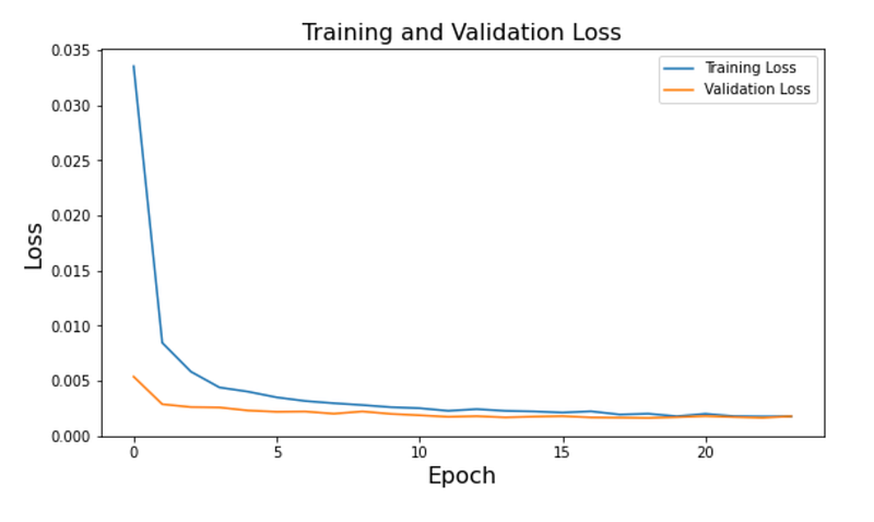
This code generates a plot that visualizes the training and validation loss of a machine learning model as it trains. It uses the matplotlib library to create a figure of a specific size and then sets up a subplot with two columns. The code creates a plot using training loss and validation loss values saved in the history object. The plot is customized with labels, a legend, axes labels, a title, and adjusts the y-axis limits based on the maximum loss value in the data. The plot is shown on the screen, allowing users to see how the loss values change throughout the training epochs.
Predicting using the trained LSTM model on the test data
test_predict=model.predict(x_test)This code uses an existing machine learning model, which has been trained beforehand and saved in a variable named “model.” It predicts output values by utilizing input data provided as x_test. The predicted values are then saved in a variable called test_predict. These predictions can be further examined or used to evaluate how well the model is performing.
Test data predicted shape
test_predict=scaler.inverse_transform(test_predict)
y_test_unscaled = scaler.inverse_transform(y_test)
test_predict.shape
(1478, 7)This code reverses the scaling of predicted values and true values to their original unscaled format using the scaler.inverse_transform() method. The function then returns the number of elements in the predicted values array test_predict.
Assessing performance involves analyzing how well a particular task or activity has been carried out. This evaluation helps determine the efficiency and effectiveness of individuals, teams, or processes.
RMSE, MAE, MAPE, and MDAPE computed
i = out - 1
RMSE = math.sqrt(mean_squared_error(y_test_unscaled[:, i],test_predict[:, i]))
print(f'Root Mean Square Error(RMSE): {np.round(RMSE, 2)}')
MAE = mean_absolute_error(y_test_unscaled[:, i],test_predict[:, i])
print(f'Median Absolute Error (MAE): {np.round(MAE, 2)}')MAPE = np.mean((np.abs(np.subtract(y_test_unscaled[:, i],test_predict[:, i])/ y_test_unscaled[:, i]))) * 100
print(f'Mean Absolute Percentage Error (MAPE): {np.round(MAPE, 2)} %')MDAPE = np.median((np.abs(np.subtract(y_test_unscaled[:, i],test_predict[:, i])/ y_test_unscaled[:, i])) ) * 100
print(f'Median Absolute Percentage Error (MDAPE): {np.round(MDAPE, 2)} %')Root Mean Square Error(RMSE): 58.28
Median Absolute Error (MAE): 37.69
Mean Absolute Percentage Error (MAPE): 3.5 %
Median Absolute Percentage Error (MDAPE): 2.62 %This code computes and displays various error metrics used to assess the effectiveness of a predictive model. RMSE stands for Root Mean Square Error, which is calculated by using the mean_squared_error function from the math library. RMSE helps us understand the average difference between the actual and predicted values in a model. Lower RMSE values suggest that the model performs better. The Mean Absolute Error (MAE) is computed with the mean_absolute_error function to measure the average absolute difference between actual and predicted values. Lower MAE values indicate better performance. The Mean Absolute Percentage Error (MAPE) is a measure that calculates the percentage difference between the actual and predicted values. It provides a relative error percentage compared to the actual values, with lower MAPE values indicating higher accuracy. The Median Absolute Percentage Error (MDAPE) is a way to measure the accuracy of a forecast. It is calculated as a percentage, similar to Mean Absolute Percentage Error (MAPE), but it uses the median instead of the mean. MDAPE is a more robust measure because it is less affected by outliers in the data. After performing calculations, the values for RMSE, MAE, MAPE, and MDAPE are displayed with two decimal places for better clarity. These metrics provide insight into the accuracy of the model’s predictions in comparison to the real values.
DataFrame “valid” updated with predictions
Train = data_filtered[:split]
valid = data_filtered[split:]
valid['Predictions'] = test_predict[:, out-1]
validC:\Users\MSI-1\AppData\Local\Temp\ipykernel_16360\536917190.py:3: SettingWithCopyWarning:
A value is trying to be set on a copy of a slice from a DataFrame.
Try using .loc[row_indexer,col_indexer] = value insteadSee the caveats in the documentation: https://pandas.pydata.org/pandas-docs/stable/user_guide/indexing.html#returning-a-view-versus-a-copy
valid['Predictions'] = test_predict[:, out-1]
This code divides a dataset into two parts, training and validation, based on the value stored in the variable ‘split’. The “Train” part includes data from the beginning to a certain point of separation, while the “Valid” part includes data from the separation point to the end of the dataset. The code creates a new column named ‘Predictions’ in the valid dataset. This column is filled with values retrieved from the variable test_predict[:, out-1]. These values likely represent the predictions generated by a model when applied to the validation dataset.
Model plot displayed with train, validation, and predicted values
plt.figure(figsize=(16,8 ))
plt.title('Model')
plt.xlabel('Date')
plt.ylabel('Close')

plt.plot(Train['Close'])
plt.plot(valid['Close'])
plt.plot(valid['Predictions'])

plt.legend(['Train', 'Val', 'Predictions'], loc='upper right')

plt.show()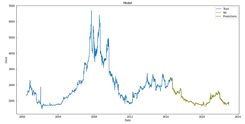
This code creates a visual representation of how well a model can predict stock prices. It produces a plot that includes the following components: The figure is 16 units wide and 8 units high. The plot is titled ‘Model’. The x-axis is labeled as ‘Date’ and the y-axis is labeled as ‘Close’. It shows the real closing prices of the training data by connecting them with a line. It shows the real closing prices of the validation data (valid[‘Close’]) by using a line on the plot. It shows the expected closing prices on the validation data by using a line graph for ‘valid[‘Predictions’]’. A legend in a plot is used to identify the lines as either ‘Train’, ‘Val’ (Validation), or ‘Predictions’. The plot displays the closing prices of the stock data, both actual and predicted.
Actual vs Predicted plot on test data displayed
plt.figure(figsize=(16,8))
plt.title("Actual vs Predicted on test data")
plt.plot(valid['Close'])
plt.plot(valid['Predictions'])
plt.xlabel('Date')
plt.ylabel('Close Price')
plt.show()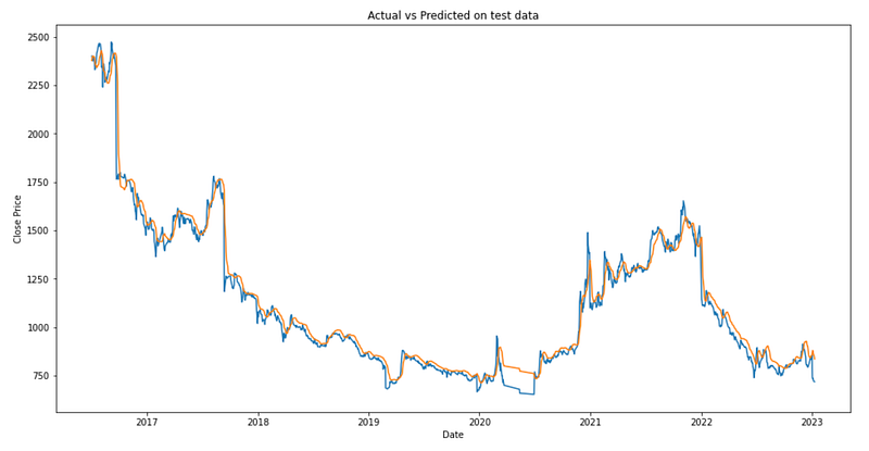
This code generates a 16x8-inch graph. It plots two lines: one for the actual ‘Close’ prices from test data and another for the predicted ‘Close’ prices. The x-axis is ‘Date’ and the y-axis is ‘Close Price’. It visualizes how closely the model’s predictions align with the actual data.


