A Surprising Way to Smoothen a Time Series — Solving the Heat Equation!

With an application to smoothening out financial market data

When developing machine learning models for time-series pattern recognition, I like to pre-process my data so that it is smoother. This sometimes help speed up convergence since the algorithm may better understand any trends or features. I have in the past used the following approaches:

1. Calculating moving averages — an simple method and pretty quick to calculate; but it means that your time series will be lagged (see the image below).
2. Methods like the Savitzky-Golay filter which fits local polynomials of degree n to each datapoint, using a fixed window of m datapoints.

To illustrate, here are the two above examples on some of TLSA’s recent stock-price history:

But wait! There is another method we can use — that of solving Partial Differential Equations (PDEs). Since I have a background in the analytical/numerical solutions of PDEs (part of my PhD was on such a topic), I figured why not merge these skills with data-science (where I currently work). Throughout this article, I will cover the following:

• Solving the heat equation numerically using a basic finite difference approach to smoothen a time series.
• The advantages and disadvantages of using this method over the beforementioned approaches.
• The application of this to stock-market data, purely because this type of data is notoriously noisy (and I find finance quite interesting!).
• Potential extensions on this work for further improvements.

Enough chat, let’s see some mathematics and code!

The Heat Equation and Why We Are Using It

First of all, what is the heat equation? Well, in simple terms, it’s this:

But, if you’re a normal human being and can’t read equations like your native language, then here it is English.

The heat equation describes the rate of diffusivity of heat through a medium. The second law of thermodynamics says that heat will flow from hotter areas into nearby colder areas, and thus, we solve the heat equation to understand this heat propagation.

This is clearly a very basic explanation, this article by Panda the Red describes the more nitty gritty of the equation for those who are interested.

But if we are considering time-series processing, we are not interested in finding the propagation of heat throughout a medium… so why use it? Well, the effect of heat propagating from warmer to cooler spots essentially acts as an averaging, or smoothening feature, this is what is useful to us.

To illustrate, I have solved the heat equation numerically for a portion of TSLA’s stock history (using the closing prices) until t=30, in steps of 0.1. You can see the smoothening effect from the heat equation in the GIF below:

Now that we are introduced to the heat equation, let’s crack on with solving it for the example in the GIF above.

Solving the Heat Equation Numerically

First of all, we need to define the problem mathematically, that means the heat equation and the appropriate conditions required to solve it for our problem. Since we have a PDE that’s second order in space, and first order in time, we require two boundary conditions and a single initial condition.

What this basically says is that our initial start is the stock-prices, and that our smoothed time-series remains the same at the start/end of the interval we are considering. There are plenty of adequate numerical methods one could choose to solve such a system, but arguably the most simple for our purposes is to use finite differences. This involves splitting up our domain into discrete parts, below is an illustration of what this means in 1D:

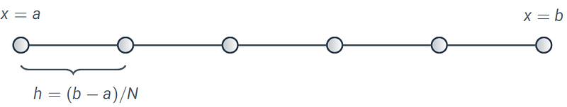
For our stock price example, each discrete component is one day, and the value at the discrete part is the closing price of that day; we will be smoothening the time-series across each of these discrete points. The discrete forms of the derivatives can be approximated as follows

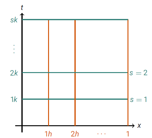
which gives a first-order accurate approximation in time, and a second-order accurate approximation in space. Here k is the step-size in time (basically, the length between each discrete point in time), and h is the step-size in space. In our example h = 1 since we have components spread apart at spaces of 1 day. Therefore, we solve for discrete points over a 2D grid, where one dimension is space, and the other is time. Below is an image to illustrate.

These approximations to the derivatives can be substituted into our PDE, and re-arranged to give

Easy stuff! It’s worth noting that for this simple explicit scheme, you only have numerical stability for 0 ≤ k ≤ 1, and the scheme will only converge if k ≤ 1/2 (the analysis to find these values is beyond the scope of this article, and involves some more complicated mathematics). You can use implicit methods which are always stable, but that’s a little more complicated and requires matrix inversions (i.e. more complex and slower!). We will use k=0.1, which is good enough for accuracy/convergence and it’s numerically stable. For those who are curious, here is what happens if you take k = 1.000000000001:

The finite difference scheme can be easily programmed in Python, here is an example below which downloads the latest stock data for TSLA using the yfinance package and plots the closing prices along with the smoothened time-series for the most recent 100 days of trading activity.

Why Use This Approach?

It’s a good question! There are other great methods to smoothen out time-series data, so why reinvent the wheel? At first I was only doing this project because I was curious to see how well it would work, but as I was working on it I noticed a few advantages:

1. This method has less parameters than the Savitzky Golay filter — no need to worry about the window size and polynomial order (which may be tricky to visualise/understand), this approach only requires you to set a finishing time.
2. I found it intuitive — the first number of time-steps filters out any high-frequency noise, then the macro-scale features are smoothened. This means you simply adjustt_end suit your pre-processing needs.
3. It was pretty quick on some speed tests I ran, provided you wrap the function in a @numba.jit(nopython = True) decorator (more on this below).

The disadvantages are:

1. The method is simple, and improving it would require using more complex finite-difference schemes and/or modify the heat-equation to make it non-linear (see, e.g., the Perona-Malik equation).
2. You have to have a good understanding of finite-differences to not encounter any problems such as numerical stability.
3. Technically, the finite difference scheme is not accurate in space because our step-size, h, is rather large. Ideally we want h to be 0.1 or less for some degree of accuracy. However, as the GIF example shows, the scheme is good enough to do what we want.

You can fix disadvantage #3 by using the analytical solution which is determined using the method of Separation of Variables (a method of solving linear PDEs). The solution in our notation is as follows:

I did code this up too (using the trapezium rule to calculate the integrals numerically), but it wasn’t any quicker than the finite-difference approach, and the code is definitely harder to read (although, you can judge that for yourself!)

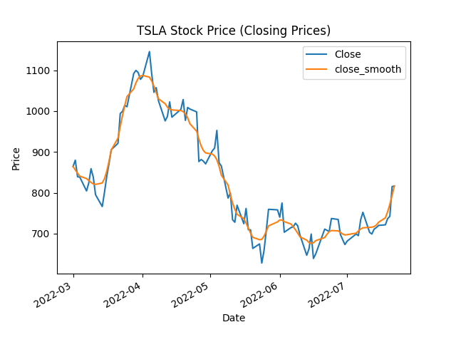
Enough mathematics… Let’s see the TSLA example once more, with the heat equation smoothened time-series included:

Not bad! The curve has roughly the same appearances as the Savitzky-Golay filter. If the heat equation is solved a smaller value of t, then the curves would be even more similar. By the way, the chart has been embedded through using Datapane, so it should be interactive!

An Example/Speed Test

For those who are interested, below is some code which pre-processes closing price time-series of 100 days in length ready for a classification/prediction algorithm. This code reformats the dataframe of prices such that each row contains 100 days of closing prices (including that date’s price), and drops the other prices and trading volume. The purpose for reformatting like this is so that we smoothen each of the time-series individually. If we applied the method to the whole of the stock’s history at once, then each point is smoothed in relation to its neighbours; therefore, when chopping it into smaller segments after processing we introduce accidental feed-forward bias. This is particularly important to avoid if you are creating a predictive algorithm!

On my mid-range laptop, the heat-equation approach took ~1.7 seconds, whereas the Savitzky Golay filter took ~4.43 seconds; this was for roughly 10,000 time-series (so you can imagine how this scales when you add more!).

Wrapping Up

In this article, we have looked into how we can harness the power of PDEs and mathematics to smoothen out time-series, specifically applied to stock-market data. Besides the more traditional approaches, the finite-difference solution presented here works pretty well, and it’s fairly fast too! I’m certain that the method can be further developed to be even quicker, or to include non-linear terms in the PDE so that edges can be preserved better (see here for an example of the Perona-Malik PDE).

I hope you enjoyed the article, or found some of it useful for your applications! This is definitely the most mathsy post I have done so far, so well done if you read it all without skipping anything! Please leave a clap if you read all the article, or, if you don’t want to publicly admit you like maths/PDEs, then let me know on LinkedIn. Also feel free to follow/DM me on twitter. 🙂

Also — this article has now been moved to my personal website, that one will be maintained and developed on further in the future 🙂

If you are thinking getting a medium account, then please consider supporting me and thousands of other writers by singing up for a membership. For full disclosure, singing up through this link grants me a portion of your membership fee, at no additional cost to you (a win-win for sure!).

Or if you’d like another way to support my content creation, then you could

Because I work a full-time job, go to the gym, trade, and write on Medium, I use a lot of coffee!