A Step-by-Step Guide to Speech Recognition and Audio Signal Processing in Python

The Science of Teaching Human Vocabulary to Machines

Speech is the primary form of human communication and is also a vital part of understanding behavior and cognition. Speech Recognition in Artificial Intelligence is a technique deployed on computer programs that enables them in understanding spoken words.

As images and videos, sound is also an analog signal that humans perceive through sensory organs.

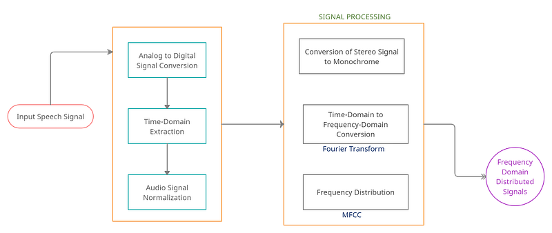
For machines, to consume this information, it needs to be stored as digital signals and analyzed through software. The conversion from analog to digital consists of the below two processes:

1. Sampling: It is a procedure used to convert a time-varying (changing with time) signal s(t) to a discrete progression of real numbers x(n). Sampling period (Ts) is a term that defines the interval between two successive discrete samples. Sampling Frequency (fs = 1/Ts) is the inverse of the sampling period. Common sampling frequencies are 8 kHz, 16 kHz, and 44.1 kHz. A 1 Hz sampling rate means one sample per second and therefore high sampling rates mean better signal quality.
2. Quantization: This is the process of replacing every real number generated by sampling with an approximation to obtain a finite precision (defined within a range of bits). In the majority of scenarios, 16 bits per sample are used for the representation of a single quantized sample. Therefore, raw audio samples generally have a signal range of -215 to 215 although, during analysis, these values are standardized to the range (-1, 1) for simpler validation and model training. A sample resolution is always measured in bits per sample.

A general Speech Recognition system is designed to perform the tasks mentioned below and can easily be correlated with a standard data analytics architecture:

1. The capture of speech (words, sentences, phrases) given by a human. You can think of this as the Data Acquisition part of any general Machine Learning workflow.
2. Transforming audio frequencies to make it machine-ready. This process is the data pre-processing part where we clean features of the data for the machine to process it.
3. Application of Natural Language Processing (NLP) on the acquired data to understand the content of speech.
4. Synthesis of the recognized words to help the machine speak a similar dialect.

Let us walk through all these steps and processes one by one, in detail, with the corresponding pseudo-code. Also, before we start, below is a link for the complete code repository that will be handy to go through alongside this tutorial.

Step 1: Reading a File for Audio Signals

File I/O in Python (scipy.io): SciPy has numerous methods of performing file operations in Python. The I/O module that includes methods read(filename[, mmap]) and write(filename, rate, data) is used to read from a .wav file and write a NumPy array in the form of a .wav file. We will be using these methods to read from and write to sound (audio) file formats.

The first step in starting a speech recognition algorithm is to create a system that can read files that contain audio (.wav, .mp3, etc.) and understanding the information present in these files. Python has libraries that we can use to read from these files and interpret them for analysis. The purpose of this step is to visualize audio signals as structured data points.

• Recording: A recording is a file we give to the algorithm as its input. The algorithm then works on this input to analyze its contents and build a speech recognition model. This could be a saved file or a live recording, Python allows for both.
• Sampling: All signals of a recording are stored in a digitized manner. These digital signatures are hard for software to work upon since machines only understand numeric input. Sampling is the technique used to convert these digital signals into a discrete numeric form. Sampling is done at a certain frequency and it generates numeric signals. Choosing the frequency levels depends on the human perception of sound. For instance, choosing a high frequency implies that the human perception of that audio signal is continuous.

# Using IO module to read Audio Files
from scipy.io import wavfile
freq_sample, sig_audio = wavfile.read("/content/Welcome.wav")

# Output the parameters: Signal Data Type, Sampling Frequency and Duration
print('\nShape of Signal:', sig_audio.shape)
print('Signal Datatype:', sig_audio.dtype)
print('Signal duration:', round(sig_audio.shape[0] / float(freq_sample), 2), 'seconds')
>>> Shape of Signal: (645632,) 
>>> Signal Datatype: int16 
>>> Signal duration: 40.35 seconds

# Normalize the Signal Value and Plot it on a graph
pow_audio_signal = sig_audio / np.power(2, 15)
pow_audio_signal = pow_audio_signal [:100]
time_axis = 1000 * np.arange(0, len(pow_audio_signal), 1) / float(freq_sample)

plt.plot(time_axis, pow_audio_signal, color='blue')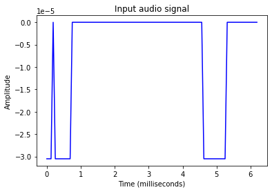

This is the representation of the sound amplitude of the input file against its duration of play. We have successfully extracted numerical data from an audio (.wav) file.

Step 2: Transforming Audio Frequencies

The representation of the audio signal we did in the first section represents a time-domain audio signal. It shows the intensity (loudness or amplitude) of the sound wave with respect to time. Portions with amplitude = 0, represent silence.

In terms of sound engineering, amplitude = 0 is the sound of static or moving air particles when no other sound is present in the environment.

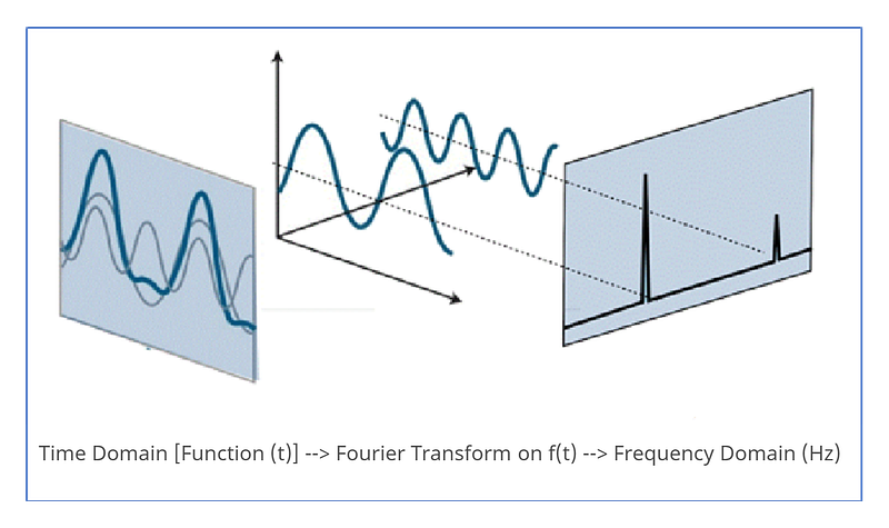
Frequency-Domain Representation: To better understand an audio signal, it is necessary to look at it through a frequency domain. This representation of an audio signal will give us details about the presence of different frequencies in the signal. Fourier Transform is a mathematical concept that can be used in the conversion of a continuous signal from its original time-domain state to a frequency-domain state. We will be using Fourier Transforms (FT) in Python to convert audio signals to a frequency-centric representation.

Fourier Transforms in Python: Fourier Transforms is a mathematical concept that can decompose this signal and bring out the individual frequencies. This is vital for understanding all the frequencies that are combined together to form the sound we hear. Fourier Transform (FT) gives all the frequencies present in the signal and also shows the magnitude of each frequency.

All audio signals are composed of a collection of many single-frequency sound waves that travel together and create a disturbance in the medium of movement, for instance, a room. Capturing sound is essentially the capturing of the amplitudes that these waves generated in space.

NumPy (np.fft.fft): This NumPy function allows us to compute a 1-D discrete Fourier Transform. The function uses Fast Fourier Transform (FFT) algorithm to convert a given sequence to a Discrete Fourier Transform (DFT). In the file we are processing, we have a sequence of amplitudes drawn from an audio file, that were originally sampled from a continuous signal. We will use this function to covert this time-domain to a discrete frequency-domain signal.

Let us now walk through some code to implement Fourier Transform to Audio signals with the aim of representing sound to its intensity (decibels (dB))

# Working on the same input file
# Extracting the length and the half-length of the signal to input to the foruier transform
sig_length = len(sig_audio)
half_length = np.ceil((sig_length + 1) / 2.0).astype(np.int)

# We will now be using the Fourier Transform to form the frequency domain of the signal
signal_freq = np.fft.fft(sig_audio)

# Normalize the frequency domain and square it
signal_freq = abs(signal_freq[0:half_length]) / sig_length
signal_freq **= 2
transform_len = len(signal_freq)

# The Fourier transformed signal now needs to be adjusted for both even and odd cases
if sig_length % 2:
  signal_freq[1:transform_len] *= 2
else:
  signal_freq[1:transform_len-1] *= 2

# Extract the signal's strength in decibels (dB)
exp_signal = 10 * np.log10(signal_freq)
x_axis = np.arange(0, half_length, 1) * (freq_sample / sig_length) / 1000.0

plt.plot(x_axis, exp_signal, color='green', linewidth=1)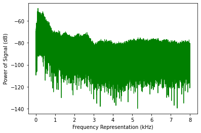

With this, we were able to apply Fourier Transforms to the Audio input file and subsequently see a frequency domain (frequency against signal strength) representation of the audio.

Step 3: Extracting Features from Speech

Once the speech is moved from a time-domain signal to a frequency domain signal, the next step is to convert this frequency domain data into a usable feature vector. Before starting this, we have to know about a new concept called MFCC.

Mel Frequency Cepstral Coefficients (MFCCs)

MFCC is a technique designed to extract features from an audio signal. It uses the MEL scale to divide the audio signal’s frequency bands and then extracts coefficients from each individual frequency band, thus, creating a separation between frequencies. MFCC uses the Discrete Cosine Transform (DCT) to perform this operation. The MEL scale is established on the human perception of sound, i.e., how the human brain process audio signals and differentiates between the varied frequencies. Let us look at the formation of the MEL scale below.

• Human voice sound perception: An adult human, has a fundamental hearing capacity that ranges from 85 Hz to 255 Hz, and this can further be distinguished between genders (85Hz to 180 Hz for Male and 165 Hz to 255 Hz for females). Above these fundamental frequencies, there also are harmonics that the human ear processes. Harmonics are multiplications of the fundamental frequency. These are simple multipliers, for instance, a 100 Hz frequency’s second harmonic will be 200 Hz, third would be 300 Hz, and so on.

The rough hearing range for humans is 20Hz to 20KHz and this sound perception is also non-linear. We can distinguish low-frequency sounds better in comparison to high-frequency sounds. For example, we can clearly state the difference between signals of 100Hz and 200Hz but cannot distinguish between 15000 Hz and 15100 Hz. To generate tones of varied frequencies we can use the program above or use this tool.

• MEL Scale: Stevens, Volkmann, and Newmann proposed a pitch in 1937 that introduced the MEL scale to the world. It is a pitch scale (scale of audio signals with varying pitch levels) that is judged by humans on the basis of equality in their distances. It is basically a scale that is derived from human perception. For example, if you were exposed to two sound sources distant from each other, the brain will perceive a distance between these sources without actually seeing them. This scale is based on how we humans measure audio signal distances with the sense of hearing. Because our perception is non-linear, the distances on this scale increase with frequency.
• MEL-spaced Filterbank: To compute the power (strength) of every frequency band, the first step is to distinguish the different feature bands available (done by MFCC). Once these segregations are made, we use filter banks to create partitions in the frequencies and separate them. Filter banks can be created using any specified frequency for partitions. The spacing between filters within a filter bank grows exponentially as the frequency grows. In the code section, we will see how to separate frequency bands.

Mathematics of MFCCs and Filter Banks

MFCC and the creation of filter banks are all motivated by the nature of audio signals and impacted by the way in which humans perceive sound. But this processing also requires a lot of mathematical computation that goes behind the scenes in its implementation. Python directly gives us methods to build filters and perform the MFCC functionality on sound but let us glance at the maths behind these functions.

Three discrete mathematical models that go into this processing are the Discrete Cosine Transform (DCT), which is used for decorrelation of filter bank coefficients, also termed as whitening of sound, and Gaussian Mixture Models — Hidden Markov Models (GMMs-HMMs) that are a standard for Automatic Speech Recognition (ASR) algorithms.

Although, in the present day, when computation costs have gone down (thanks to Cloud Computing), deep learning speech systems that are less susceptible to noise, are used over these techniques.

DCT is a linear transformation algorithm, and it will therefore rule out a lot of useful signals, given sound is highly non-linear.

# Installing and importing necessary libraries
pip install python_speech_features
from python_speech_features import mfcc, logfbank
sampling_freq, sig_audio = wavfile.read("Welcome.wav")

# We will now be taking the first 15000 samples from the signal for analysis
sig_audio = sig_audio[:15000]

# Using MFCC to extract features from the signal
mfcc_feat = mfcc(sig_audio, sampling_freq)
print('\nMFCC Parameters\nWindow Count =', mfcc_feat.shape[0])
print('Individual Feature Length =', mfcc_feat.shape[1])
>>> MFCC Parameters Window Count = 93 
>>> Individual Feature Length = 13

mfcc_feat = mfcc_feat.T
plt.matshow(mfcc_feat)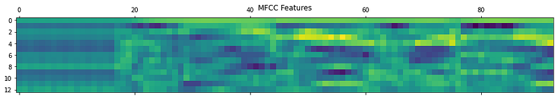

# Generating filter bank features
fb_feat = logfbank(sig_audio, sampling_freq)
print('\nFilter bank\nWindow Count =', fb_feat.shape[0])
print('Individual Feature Length =', fb_feat.shape[1])
>>> Filter bank Window Count = 93
>>> Individual Feature Length = 26

fb_feat = fb_feat.T
plt.matshow(fb_feat)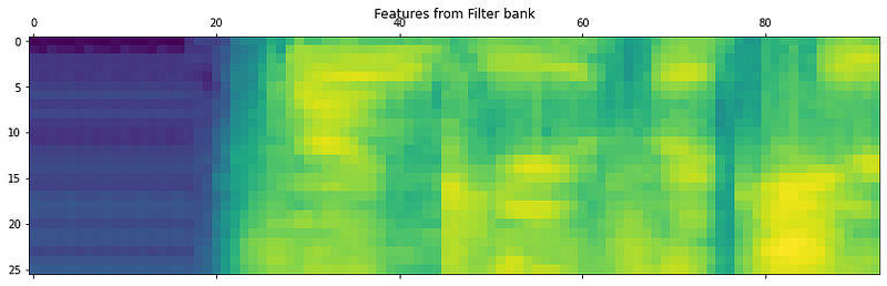

If we see the two distributions, it is evident that the low frequency and high-frequency sound distributions are separated in the second image.

The MFCC, along with application of Filter Banks is a good algorithm to separate the high and low frequency signals. This expedites the analysis process as we can trim sound signals into two or more separate segments and individually analyze them based on their frequencies.

Step 4: Recognizing Spoken Words

Speech Recognition is the process of understanding the human voice and transcribing it to text in the machine. There are several libraries available to process speech to text, namely, Bing Speech, Google Speech, Houndify, IBM Speech to Text, etc. We will be using the Google Speech library to convert Speech to Text.

Google Speech API

More about the Google Speech API can be read from the Google Cloud Page and the Speech Recognition PyPi page. A few key features that the Google Speech API is capable of are the adaptation of speech. This means that the API understands the domain of the speech. For instance, currencies, addresses, years are all prescribed into the speech-to-text conversion. There are domain-specific classes defined in the algorithm that recognize these occurrences in the input speech. The API works with both on-prem, pre-recorded files as well as live recordings on the microphone in the present working environment. We will analyze live speech through microphonic input in the next section.

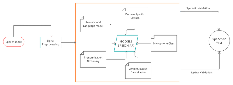
1. Working with Microphones: The PyAudio open-source package allows us to directly record audio through an attached microphone and analyze it with Python in real-time. The installation of PyAudio will vary based on the operating system (the installation explanation is mentioned in the code section below).
2. Microphone Class: The instance of the .microphone() class can be used with Speech Recognizer to directly record audio within the working directory. To check if microphones are available in the system, use the list_microphone_names static method. To use any of the available listed microphones use the device_index method (Implementation shown in the code below)
3. Capturing Microphone Input: The listen() function is used to capture input given to the microphone. All the sound signals that the selected microphone receives, are stored in the variable that calls the listen() function. This method continues recording until a silent ( 0 amplitude) signal is detected.
4. Ambient Noise Reduction: Any functional environment is prone to have ambient noise that will hamper the recording. Therefore, the adjust_for_ambient_noise() method within the Recognizer class helps automatically cancel out ambient noise from the recording.
5. Recognition of Sound: The speech recognition workflow below explains the part after processing of signals where the API performs tasks like Semantic and Syntactic corrections, understands the domain of sound, the spoken language, and finally creates the output by converting speech to text. Below we will also see the implementation of Google’s Speech Recognition API using the Microphone class.

# Install the SpeechRecognition and pipwin classes to work with the Recognizer() class
pip install SpeechRecognition
pip install pipwin

# Below are a few links that can give details about the PyAudio class we will be using to read direct microphone input into the Jupyter Notebook
# https://anaconda.org/anaconda/pyaudio
# https://www.lfd.uci.edu/~gohlke/pythonlibs/#pyaudio
# To install PyAudio, Run in the Anaconda Terminal CMD: conda install -c anaconda pyaudio
# Pre-requisite for running PyAudio installation - Microsoft Visual C++ 14.0 or greater will be required. Get it with "Microsoft C++ Build Tools" : https://visualstudio.microsoft.com/visual-cpp-build-tools/
# To run PyAudio on Colab, please install PyAudio.whl in your local system and give that path to colab for installation

pip install pyaudio
import speech_recognition as speech_recog

# Creating a recording object to store input
rec = speech_recog.Recognizer()

# Importing the microphone class to check availabiity of microphones
mic_test = speech_recog.Microphone()

# List the available microphones
speech_recog.Microphone.list_microphone_names()

# We will now directly use the microphone module to capture voice input. Specifying the second microphone to be used for a duration of 3 seconds. The algorithm will also adjust given input and clear it of any ambient noise

with speech_recog.Microphone(device_index=1) as source: 
    rec.adjust_for_ambient_noise(source, duration=3)
    print("Reach the Microphone and say something!")
    audio = rec.listen(source)

>>> Reach the Microphone and say something!

# Use the recognize function to transcribe spoken words to text
try:
    print("I think you said: \n" + rec.recognize_google(audio))
except Exception as e:
    print(e)
>>> I think you said: 
>>> hi hello hello hello

With this, we bring an end to our Speech Recognition and Sound Analysis article. I would still advise you to go through the links mentioned in the References section and the code repository linked at the top of the story to be able to follow it at every step.

THAT’S A WRAP!

Conclusion

Speech recognition is an AI concept that allows a machine to listen to a human voice and transcribe text out of it. Although complex in nature, the use cases revolving around Speech Recognition are plenty. From helping differently-abled users with access to computing to an automated response machine, Automatic Speech Recognition (ASR) algorithms are being used by many industries today. This chapter gave a brief introduction to the engineering of sound analysis and showed some basic manipulation techniques to work with audio. Though not detailed, it will help in creating an overall picture of how speech analysis works in the world of AI.

About Me

I am Rahul, currently researching Artificial Intelligence and implementing Big Data Analytics on Xbox Games. I work with Microsoft. Apart from professional work, I am also trying to work out a program that deals with understanding how economic situations can be improved across developing nations in the world by using AI.

I am at Columbia University in New York at the moment and you are free to connect with me on LinkedIn on Twitter.

[References]

1. https://www.ibm.com/cloud/learn/speech-recognition
2. https://www.sciencedirect.com/topics/engineering/speech-recognition
3. https://signalprocessingsociety.org/publications-resources/blog/what-are-benefits-speech-recognition-technology
4. https://www.analyticsvidhya.com/blog/2021/01/introduction-to-automatic-speech-recognition-and-natural-language-processing/
5. https://cloud.google.com/speech-to-text
6. https://www.analyticsvidhya.com/blog/2021/06/mfcc-technique-for-speech-recognition/
7. https://www.google.com/intl/en/chrome/demos/speech.html
8. https://ocw.mit.edu/courses/electrical-engineering-and-computer-science/6-345-automatic-speech-recognition-spring-2003/lecture-notes/lecture5.pdf
9. https://towardsdatascience.com/understanding-audio-data-fourier-transform-fft-spectrogram-and-speech-recognition-a4072d228520
10. https://haythamfayek.com/2016/04/21/speech-processing-for-machine-learning.html