A Simple Indicator to Add to Your Trading System

Presenting a Simple Indicator Idea that should be included in your Trading Framework

Note from Towards Data Science’s editors: While we allow independent authors to publish articles in accordance with our rules and guidelines, we do not endorse each author’s contribution. You should not rely on an author’s works without seeking professional advice. See our Reader Terms for details.

Financial research is an endless exciting field with many “Eureka” and “Oh no!” moments. We always seek out that golden strategy that works all the time and makes us sleep well during the night, but we are often encountered with “Oh no!” moments. This is quite normal, we are looking for a needle in a haystack, the needle being a decent strategy and the haystack being the endless possibilities of ideas.

I have just published a new book after the success of New Technical Indicators in Python. It features a more complete description and addition of complex trading strategies with a Github page dedicated to the continuously updated code. If you feel that this interests you, feel free to visit the below link, or if you prefer to buy the PDF version, you could contact me on Linkedin.

Sometimes, simplicity is the key for success. We do not need dozens of technical indicators giving out signals here and there only to find ourselves net losers at the end of the month. We have to understand two things about technical indicators:

• They are price derived. this means that they take the price and decompose it to understand some characteristics. They are therefore not forward looking but backward looking. Our hope is for this backward relationship to continue in the future. For example, if we see a divergence on the RSI, we are hoping it causes exhaustion in prices like it usually does. This divergence does not peek at the future, it is simply a mathematical observation.
• They are unlikely to provide a winning strategy on their own. If they did, then why aren’t we all millionaires depending on overbought/oversold zones on the Stochastic indicator? Trading is much more complicated than that and requires a more thorough approach to find profitable trades.

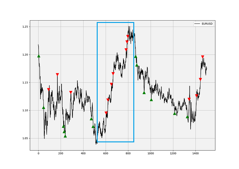
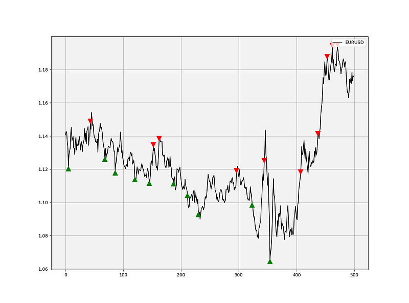
With that being in mind, we should think of indicators as little helpers with our convictions. For example, when we find sufficient information to tell us to go long (buy) an asset, we can check the technical indicators to see whether they confirm this or not. We should also check the current market state to know whether the indicator is going to provide a good signal or not. This means that we should not use mean-reverting indicators when we are in a trending market. The below graph shows why. It is the sell signals given by the RSI on an upward trending market. Notice the trending price action inside the blue rectangle, it is clear that the quality of the signals is quite bad.

Now, we can try to find a simple indicator from a very simple idea, that is, Normalization. The good news with normalization is that the buy and sell conditions are already outlined and are intuitive, hence, all we have to do is find a decent period (such as the 14 default period in the RSI). We will see how to find this period without biasing the indicator.

The Concept of Normalization

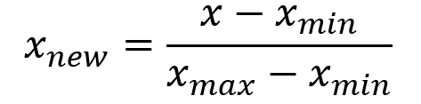
This great technique allows us to trap the values between 0 and 1 (or 0 and 100 if we wish to multiply by 100). The concept revolves around subtracting the minimum value in a certain lookback period from the current value and dividing by the maximum value in the same lookback period minus the minimum value (the same in the nominator).

We can try to code this formula in python. The below function normalizes a given time series of the OHLC type:

def normalizer(Data, lookback, onwhat, where):
        
    for i in range(len(Data)):
        
        try:
    
            Data[i, where] = (Data[i, onwhat] - min(Data[i - lookback + 1:i + 1, onwhat])) / (max(Data[i - lookback + 1:i + 1, onwhat]) - min(Data[i - lookback + 1:i + 1, onwhat]))
        except ValueError:
            pass
    
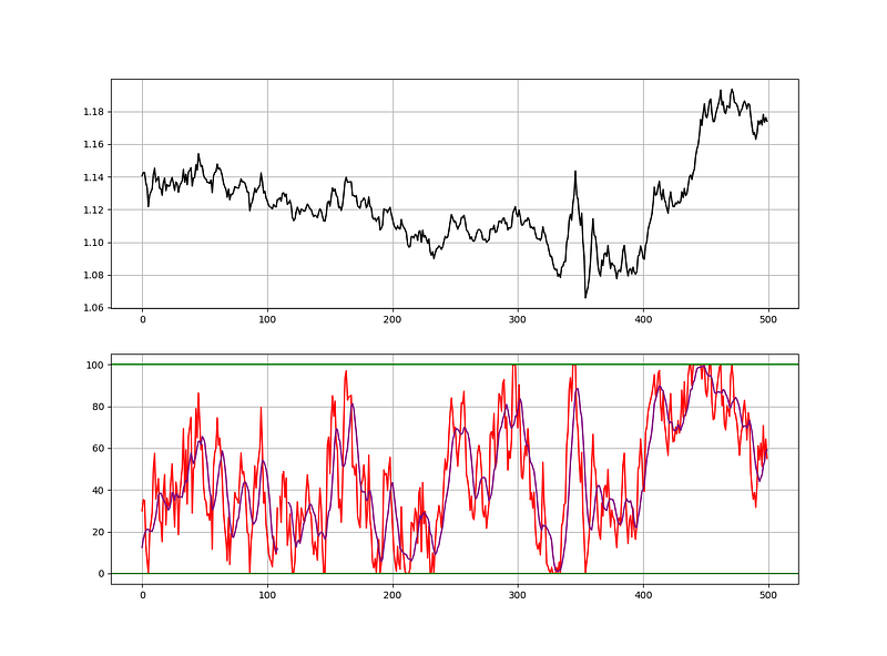
    Data[:, where] = Data[:, where] * 100

return Data

# The onwhat variable is what to normalize and the where variable is where to print the normalized values, i.e. which colum.

If we apply the function to the closing price of the EURUSD daily time frame with a 50 lookback period (meaning, the function will look at the last 50 values and select the minimum and maximum values from there) we will have the following chart.

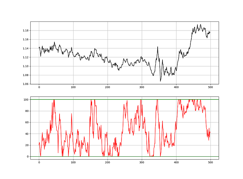
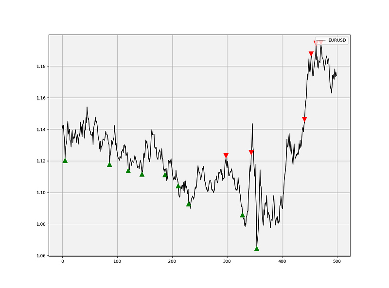
Now, if we form a simple strategy where we buy whenever the normalized value equals 0 and short whenever the normalized value equals 100, we get the below chart. The signals do seem to capture some tops and bottoms. This, on its own, is a good start as the choice of 50 was purely arbitrary. For simplicity, we can call the normalized values: The Normalized Index (NI).

If you are also interested by more technical indicators and using Python to create strategies, then my best-selling book on Technical Indicators may interest you:

However, we want to extract as much value as we can from this wonderful technique that is, Normalization. How? Here is the basic idea:

We want to eliminate the need to say that a 20-Day period is better than a 50-period for normalization and as such we can form an All-Normalized Index (ANI) that uses lookback periods from 2 to 100 and weighs them accordingly. This way we will have a weighted Normalized Index that considers the wide array of lookback periods.

If the 10-Day period Normalized Index is showing a value of 40, then its true value in the All-Normalized Index becomes 40 / 100 = 0.40. Therefore, we will have an index between 0 and 100 composed of 100 Normalized Indexers.

Speaking in Pythonic language, we will have the following statement for a loop that creates the All-Normalized Index (ANI), remember, we are still in an OHLC data structure (Column 0 for open, column 1 for high, column 2 for low, and column 3 for close):

# Starting from column 4 (i.e. the first Normalized Index)
b = 4

# Looping and adding 1 so that the correct column will be populated
for a in range(2, 102): 
  Asset1 = normalizer(Asset1, a, 3, b)
  b = b + 1

# Formatting
normalized_values = Asset1[:, 4:104]

# Calculating the ANI
all_normalizer = np.sum(normalized_values, axis=1) / 100

# Reshaping
all_normalizer = np.reshape(all_normalizer, (-1, 1))
Asset1 = deleter(Asset1, 4, 110)

# Concatenating the OHLC Data with the ANI
Asset1 = np.concatenate((Asset1, all_normalizer), axis = 1)
Asset1 = adder(Asset1, 10)
Asset1 = Asset1[102:,]

Let us see how our new indicator looks like. Spoiler alert, it looks like an indicator. By the way, if you like researching and back-testing strategies through Python, then this book I have written might interest you, The Book of Back-tests: Trading Objectively: Back-testing and Demystifying Trading Strategies.

Hence, the above indicator is an average of a hundred normalized indexers giving us signals that seem to be slightly better (we can always optimize it). Let us check the below signal chart.

We can add our touch to the ANI since the signals are a bit rare. How about adding an 8-Day moving average? That can give us some signals based on when the moving average crosses the ANI. The below chart illustrates the previous point, we have more signals and the moving average is doing a good job smoothing out the ANI.

If you are interested further in another Normalized Indicator, check out this article I have written:

Conclusion

What is the use of this indicator? Well, measuring momentum is a key concept in trading and the Normalized Index does this perfectly by using pure closing price data. If the Stochastic Oscillator uses a slightly modified version of Normalization, then the latter can help us see pure closing momentum. If you are looking to fade away a move, you can confirm your view with the ANI.

The rule of thumb is that if the ANI’s reading is higher than 95, then it is supporting your bearish view and if the ANI’s reading is lower than 5, then it is supporting your bullish view. The other way that we can use the ANI is by its moving average crossovers. Of course, the 8-period MA is a personal choice, and you can choose another period if it suits you better.