The Programmer’s Short and Practical Guide to Graph Theory

Getting started with graph theory

Graphs are very useful structures to work with in programming since very often computer science problems can be represented as a graph and solved with one of many existing graph techniques. In addition, not necessarily directly using graphs but approaching the problem through graph-based thinking and modelling can improve task clarity and efficiency.

While graph theory is a deep and fascinating field, this article will use the following sections cover broad parts of graph theory relevant to the programmer:

• Graph/node-based thinking and approaches to search problems
• Implementation of a graph with object-oriented programming
• Different representations of graphs (adjacency lists, adjacency matrices)
• Types of graphs and their implementations: un/directed graphs, un/weighted graphs, cycle graphs, a/cyclic graphs
• Dijkstra’s algorithm, weaknesses, and alternatives
• Applications of graph theory
• Summary/key points

An undirected and unweighted graph is the simplest form of a graph (besides a single node). It consists of two types of elements only: nodes, which can be thought of as points, and edges, which connect these points together. There is no idea of distance/cost or direction, which is why it is undirected and unweighted.

For instance, consider the following search problem, and represent it as an undirected and unweighted graph:

You have a padlock with two digits, initialized to 00. Each move, you can move one of the four two up or down (moving 0 up is 1, moving 0 down is 9 — the wheels are circular). There are “dead combinations,” in which the padlock will permanently lock if the combination ever equals one of those values. Find the minimum number of moves it takes to reach a target combination without locking, or if it is possible at all.

Dead combinations: [10, 90, 12]. Target: 11.

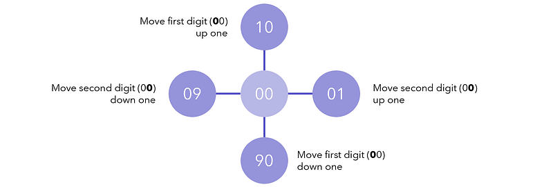
First, we construct a root, or head of the graph, which is necessary in scenarios where we need to generate the graph as we go. This is 00, or the root case from which branching cases will be generated.

The four neighbors of node 00 are 01, 10, 90, and 09, corresponding to various combinations of moving wheels up and down. Our graph already has five nodes and four edges.

For each newly added node, we will continue searching for its neighbors and add it to the graph, unless it is a dead node.

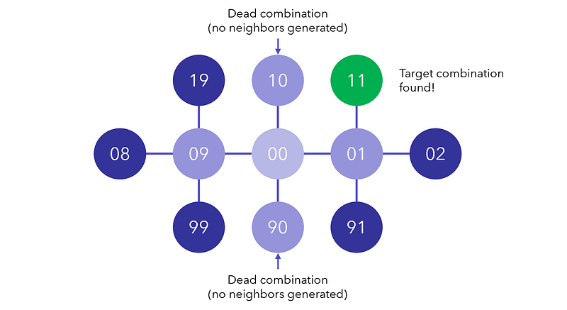
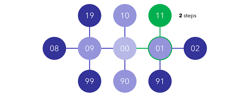
When we have found the target combination, we can retrace our steps and count how many it takes to reach the root node again. Alternatively, we could have been keeping track of the steps each time a node is generated.

If you want to implement the solution to this problem, you can use a queue and breadth-first search, which is more efficient than actually coding a graph.

This was an example of using graph-based thinking. Since graphs are very ordered and clean structures, thinking and implementing possibilities as nodes and variants as neighbors can result in a complex but clean and understandable search. Additionally, using graphs allows for many studied methods in graph theory to be implemented to speed up search.

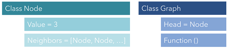
However, in this padlock problem, graphs did not actually need to be implemented. The most common method to implement a complete graph is to use two objects (classes), a Node, the primary building block, and a Graph, which is comprised of Nodes and provides an interface to access information about the graph as a whole.

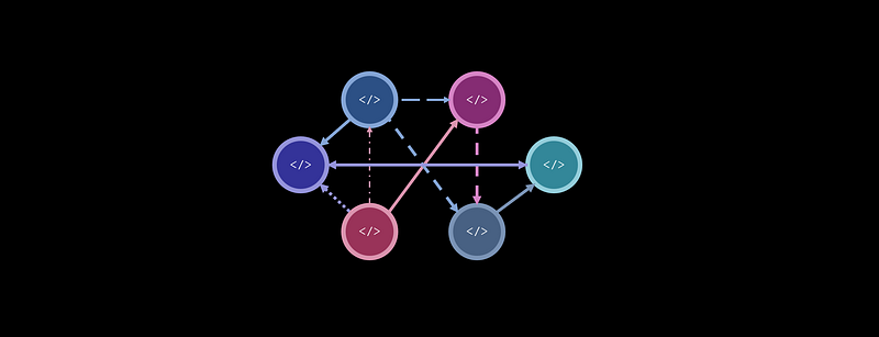
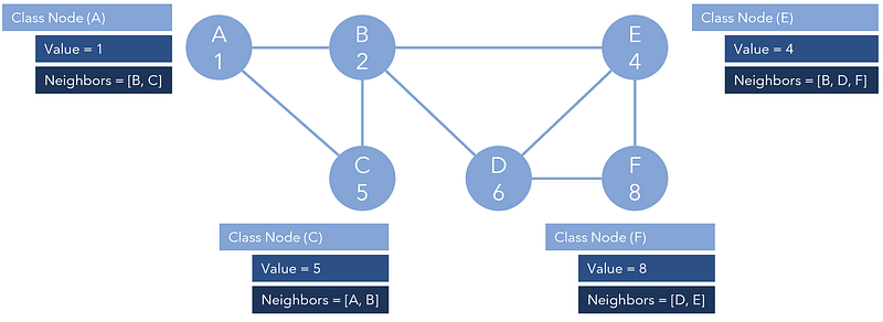
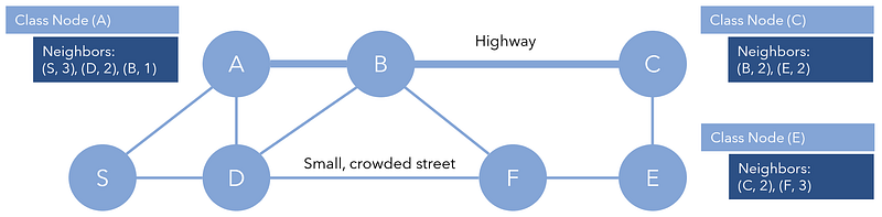
For example, each element in the graph below can be represented in code as their own Node. Each is connected to each other through their Neighbors. If we were to call something like NodeA.Neighbors[1].Neighbors[1].Value, we should receive 2. This is because the second index of Node A’s neighbors is Node C, and the second index of Node C’s neighbors is Node B, which has a value of 2. This kind of easy connectivity allows for easy traversal.

A directed graph, or a graph where edges only go in one direction, is easy to implement with this design. For example, if a one-way edge were to connect Node A to Node B, Node A’s neighbor would be Node B, but Node B would have no neighbors. Rephrased, neighbors only indicate outbound edges. Note that bidirectional edges can still exist in directed graphs.

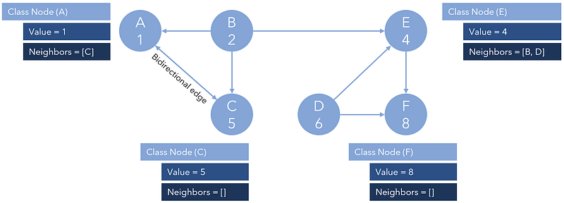
If one were to traverse the graph according to neighbors and end up at Node C or Node F, they would be stuck because those nodes have no neighbors and hence no outbound directions.

Alternatively, a graph can be represented more simply, but at the cost of being less easy to traverse, with two lists representing the edges and nodes (vertices). These are sometimes called adjacency lists since they express in list format the adjacencies between edges (adjacencies being edges and adjacent nodes being neighbors).

V = [A, B, C, D, E, F]
E = [AB, AC, BC, CF, CE, DF, EA, FB, FD]

In the example above, V declares the nodes that exist, and E declares an edge from one node to another (AC means A→C). Since it is compact and simple notation, graphs will often be presented this way.

Alternatively, it could be written as a dictionary (map), in which the key is a starting node and its value is a list of elements it points to.

adj_l = {A:[B,C], B:[C], C:[F,E], D:[F], E:[A], F:{B,D]}

Graphs, both directed and undirected, can contain loops. A cycle graph is a graph consisting of only one cycle, in which there are no terminating nodes and one could traverse infinitely throughout the graph. A cyclic graph is a graph that consists of several cycle graphs, where traversals can still be infinite but more complex.

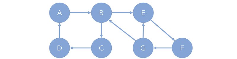
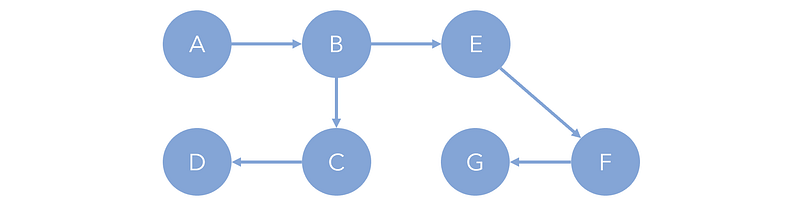
For example, within the complete cyclic graph, A→B→C→D→A is a four-cycle graph, and E→F→G→E is a three-cycle graph. More hidden is another four-cycle graph, B→E→F→G→B.

Certain types of cycles within cyclic graphs, or other components within graphs in which each node is connected to each other node, are known as strongly connected components. For instance, E→F→G→E is a strongly connected component because each of the nodes {E, F, G} has a path to another, regardless of direction. B→E→F→G→B is also a strongly connected component. On the other hand, A→B→C→D→A is not because there is no connection between component members B and D.

On the other hand, as the name suggests, acyclic graphs are ones where no cycle exists, and any traversal long enough will eventually terminate. In the graph below, no matter which node you start on, a traversal will always terminate.

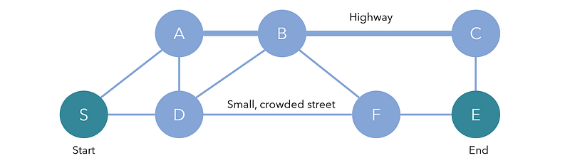
It is not always true in more complex problems that edges can naively be treated as equal to travel. For instance, if you’re planning the best route to go from a start to an end destination, you’re going to consider not only the number of segments but also the distance and the cost.

For instance, the shortest path to go from S→E is S→D→F→E, which requires only three edge traversals. However, that route takes a very small, crowded street. Alternatively, S→A→B→C→E takes four edges but travels most of the distance along a highway, and the overall cost is lessened. When the notions of distance and cost are added to a graph, it becomes weighted.

To implement this into our existing framework for graph structure, we can include for each element in Neighbors another number describing the cost to reach that neighbor. For instance, it may be stored in tuples [(n, c), (n, c)], where n represents the node and c represents the cost.

Often, graphs will also be presented in the form of a matrix, known as an adjacency matrix. This is not as compact as an adjacency list but can represent weighted graphs more naturally. In the matrix, each row and column represents a node and the cell located at (x, y) represents the edge y→x (or vice versa, it’s a matter of notation). If there is no edge, the value is 0. If there is, the value is the cost of that edge.

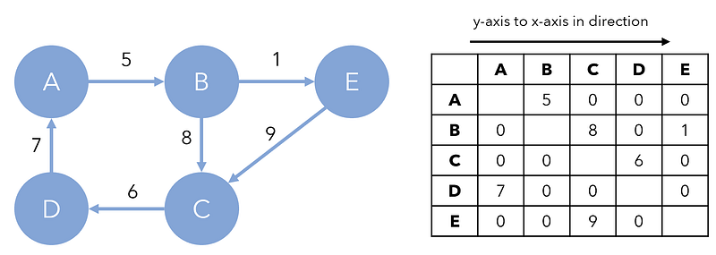
Adjacency matrices also have the advantage of easy lookup of costs, even with unweighted graphs, over adjacency lists and an object-oriented representation. Note that undirected graphs will have symmetrical adjacency matrices. Since matrices are also easier to manipulate, many graph operations and algorithms are commonly implemented on adjacency matrices.

Various algorithms have been created to find the shortest path for weighted graphs, like Dijkstra’s algorithm (pronounced dike-strah). Essentially, Dijkstra’s algorithm is very similar to the brute-force style search discussed earlier with the padlock problem but does so in a way that is most logical. The rough outline of the algorithm is as follows:

1. Begin at the start node and initialize a list (priority queue) to keep track of which nodes to process.
2. At each iteration of the algorithm, find the first element of the list. Process the element by finding all its neighboring nodes (that haven’t been explored before).
3. For each neighbor, calculate the total distance/cost to reach that node from the start node. Put these neighbor nodes into the list such that the nodes with the lowest costs are at the front.
4. Repeat until the end node has been processed.

There are plenty more in-depth resources about Dijkstra’s algorithm, but primarily, its main difference from a brute-force search is that it processes nodes currently with the smallest costs first, which is logically correct. This can speed up redundant searching by taking into account weights.

While powerful in many instances, Dijkstra is naïve in that it only chooses to process nodes that currently hold the best costs, in the hopes that the complete path will also hold a similarly small cost, when this may not be the case at all. This can be a problem in large graphs.

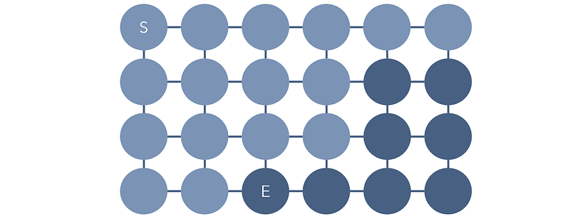
For instance, consider this grid of nodes, where each connection has the same cost to traverse; Dijkstra’s algorithm (slightly varying depending on implementation) will search through all the light nodes before arriving at the end node E. It’s like pouring a bucket of water at the location of node S and hoping it eventually spreads to the target node.

The A Star algorithm and many other variants take into account these weaknesses and add enhancements, like stronger memory and direction to improve traversals throughout graphs. Machine learning, particularly reinforcement learning, is central to more recent methods of highly efficient graph traversal. In reinforcement learning, probabilities and states are often represented as graphs an agent traverses.

Graphs and graph-based thinking can be used in many other computer science problems, even when it is not obvious. Any time you approach a difficult problem, attempting to represent it using vertices and edges can inspire new ideas, simplify and reduce the problem, or even be one solution to the problem.

Some applications of graph theory in computer science include:

• Modelling of complex networks, like social networks or in the simulation of a disease like the new coronavirus. Each node can represent one person or a population, and edges can represent probability/easiness of transmission. In this model, we can try to identify or form circular, closed graphs.
• Organization and anything hierarchical. Graphs don’t have to be loopy and cyclical; they can also express a hierarchy. For instance, if you were to create an API for a local library to access books by various content, you’d want to create a graph. If you wanted to create a site map for your website, you’d use a graph. Graph databases are types of databases that specifically rely on the graph’s organized hierarchies to store data.
• Any problem that involves an agent travelling between many locations or states is most likely represented well with a graph. Using graphs can help reduce the complexity of almost any programming problem.
• A service like Google Maps, which tells you the best route to take, considering not only distance but traffic time, elevation, tolls, etc. It is, essentially, finding the best path in a massive weighted graph (imagine a node every few feet or so, and a graph spanning the Earth).
• Graph theory was involved in the proving of the Four-Color Theorem, which became the first accepted mathematical proof run on a computer.
• In natural language processing, a division of machine learning that handles the modelling of language, weighted graph representations of words and text are extremely valuable because they can provide insight into, for example, words that belong to a similar cluster (apples, oranges) or mean similar things through distance.

Key Points

• Graphs are comprised of a set of nodes, also called vertices, and edges, or connections between the nodes.
• Two representations of graphs include adjacency lists and adjacency matrices. The latter supports easier indexing and manipulation but takes up more space than the former.
• Complete graphs can be implemented using Node objects, which have a value and a set of neighbors.
• Directed graphs have direction. Weighted graphs apply the idea of distance or cost to each edge. Cyclic graphs contain cycles that can be infinitely traversed.
• Dijkstra’s algorithm is used to find the shortest distance between two nodes in a weighted graph. It is usually effective but somewhat naïve, which is why there exists a host of other algorithms dedicated to finding the best graph traversal.
• Graphs, both in their implementation and in a thinking paradigm, can be applied to a very wide set of computer science and programming problems.