A Quick Overview of Contrast Enhancement and Its Variants for Medical Image Processing
In the last blog, I covered the pre-processing of Electron Macroscopic Images. By following the same theme of pre-processing, the basics of adaptive contrast enhancement and its application to the medical imaging will be covered in this article.
Medical images are degraded mainly because of the following two factors:
- Noise, which is inevitable during the data acquisition process.
- Low contrast, which occurs due to inconsistent illumination and several other factors.
For the further applications in medical image processing, fixing the above artifacts are necessary.
Outcomes
This blog mainly focused on the improvement of contrast in the medical images using the state-of-the-art methods as the preservation of the pixel brightness and optimal contrast are crucial for the further processing, e.g. creating the training data set in network design. Precisely, the take away points of this blog are:
- Readers will learn about the image pixel manipulations in terms of the image enhancement and de-enhancement
- An overview of the state-of-the-art transformation methods along with their effects.
- The reader will be able to pick the right transformation based on the input medical image.
Required skills:
Basics of Python and OpenCV.
Input Data
The following two image are considered for the enhancement. These images are acquired using OCT (Optical coherence tomography). The first image shows the interior surface of the eye and it includes a part of retina, optic disk (the dark circle region on right side of first image), Fovea (the bright region in the center), and Macula (regions around Fovea). The second image shows the different retinal layers in Macula region (learn more about these images).
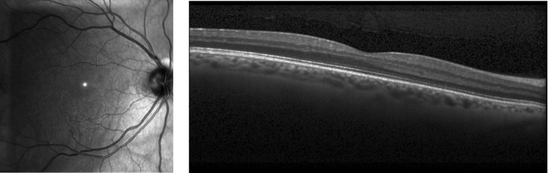
The structural analysis of the above images are vital in retinal image processing to diagnose and monitor several diseases, for example, diabetes, hypertension, strokes, and several other neurological diseases (learn more about “The eye as a window to the brain”).
In the above images have different kinds of structures and information. For example, The blood vessels and veins in the first image and retinal layers thickness in the second image.
We are not performing the full pipeline of these structures extraction in this blog. However, we will cover the initial part of the pipeline, which is the image enhancement.
Theory and Implementation
Contrast enhancement: is defined as the manipulation and redistributing the image pixels in a linear or non-linear fashion to improve the separation of obscured structural variations in pixel intensity into a more visually differentiable structural distribution.
Let us consider a low contrast image and the corresponding enhanced image, which are shown below with corresponding notations. The term xᵢ and yᵢ (i = 0, 1,…,N-1) show the pixel intensities of the corresponding images. Each image has N number of pixels with L different grey levels.
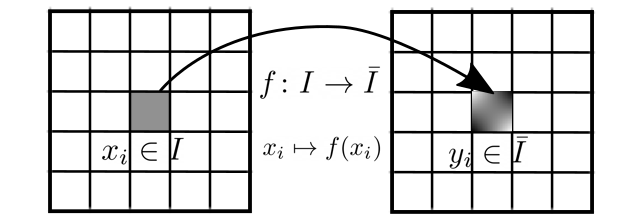
As it is mentioned above, the contrast enhancement is image manipulation and a specific manipulation can be defined by a function f, which maps a pixel from input to the corresponding output and known as transformation function.
The outcome pixel modification depends the function f, which is also responsible for the histogram modification of the input image.
To understand better the effect of the transformation function, the user should also check the distribution of the pixels in the input and output images. The distribution of the pixels can be computed using histogram, which indicates the probability distribution of the grey levels (pixels) in the image.
The histogram and non-normalized cumulative distribution (discrete mass distribution/CDF) function of a particular grey level l ( xᵢ , keep in mind that more than one pixels can have same grey level) is defined as:

where nₗ represents the number with grey level l and C(l) shows the cumulative distribution up to the grey level l. In the following, The effects of different transformation functions are shown in terms contrast enhancement/de-enhancement and histogram modifications.
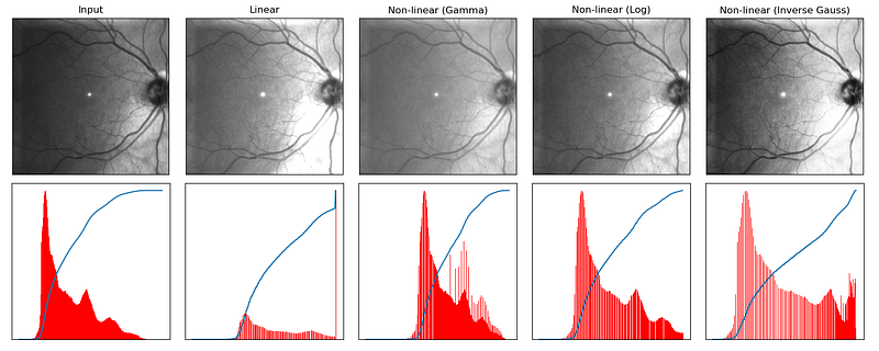
- Linear contrast enhancement: The linear transformation function is simplest way of image manipulation and it can be written as:

where the terms α and β are contrast enhancement and brightness factors respectively. As it can be seen from the above equation, the pixel intensities are changing linearly, which will increase the gradient in the whole image if α is greater than 1. The term β will improve the brightness in the image as shown in Figure 2 (second column). Due to the linear transformation, the output images can have more saturated pixels.
From histogram point of view, it is clear that this method is stretching the distribution of grey levels in the whole grey levels range.
2. Non-linear contrast enhancement (Gamma correction): To avoid over brightness in the output image, the concept of non-linear transformation function was used. The outcomes of these functions also depend on the original input pixels, however they do not simply scale the pixel values but change it according to defined function and these functions are chosen based on the input image.
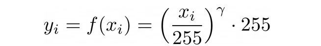
The above equation shows the Gamma correction transformation function, which computes the output pixel using power of γ to the corresponding input pixel.
The value of γ has vital part in the contrast enhancement, when γ<1, the dark pixels will be converted into bright pixels and vice versa.
From the outcome point of view, this function generates better results and a slightly modified histogram compared to the linear transformation function (Fig. 2, third column).
The other well known transformation function is the Logarithmic correction which is defined as:

where α is the scaling/gain factor.
The outcomes regarding the log transformation is shown in Fig. 2 and the similarities between gamma and log transformations are quite visible.
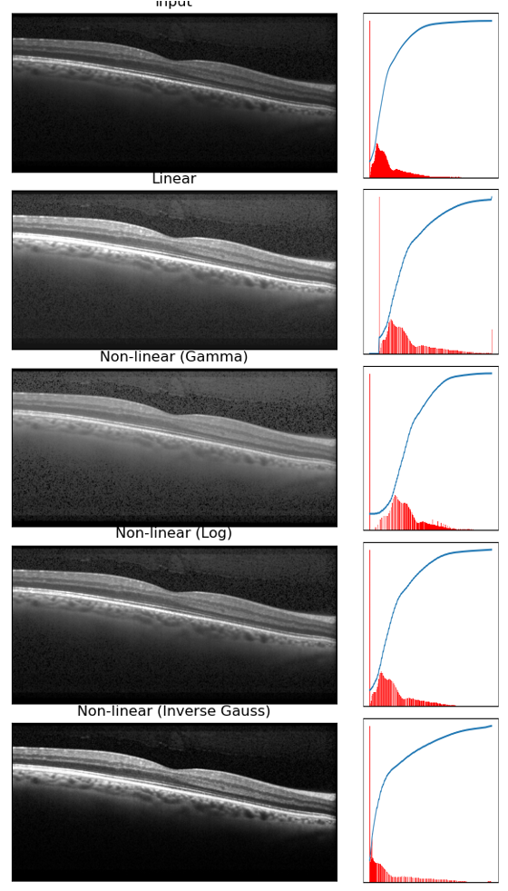
Inverted-Gauss based contrast enhancement: The user can also define an application specific transformation function according to the input image. As it can be seen from Figure 1, the left side of the pixel intensities are too low and the right side of the image has proper intensities of the pixel. Therefore to improve overall contrast of the image following function can be applied:

where σ controls the shape of the Gaussian kernel. The above function is inverted Gaussian function and the corresponding outcomes are shown in Fig 2 (last column), which is also not good as Gamma transformation method.
However, Fig. 3 shows the outcome of the above mention method with the second image of Fig 1. As it can be seen, the inverted Gaussian function performs much better compared to other methods. In the last row of Fig.3, the layers are having better contrast compared to other rows of the image
3. Histogram Equalization:
The histogram equalization improves the contrast of the input image by stretching the histogram distributions between 0 to L-1 gray levels. In other words, the transformation function f distributes the histograms equally in the whole grey level domain. Therefore, the transformation function is basically converting the cumulative histogram in a linear function .
In HE, the outcome pixel value will be proportional to the histogram of the particular grey level in the input image.

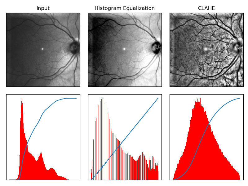
where, l is the grey level of pixel iᵗʰ pixel (xᵢ). From the above definition, it is pretty clear that the histogram equalization is not suitable for the image which has a lot of similar grey levels. For example, Fig. 4 has the retinal layer image and most the background pixel are closed to the zero (same grey levels). As it can be seen (Fig 4, second row), the layer pixels are over-bright, which is not desirable in further processing. The output histogram confirms that the transformation function mapped the CDF function into a linear function. Similarly, in Fig 5, some parts of image are too dark to see the vessel structure.
4. Adaptive Histogram Equalization: To avoid the problem of over enhancement, the concept of Adaptive Histogram Equalization (AHE) was introduced. AHE is performing enhancement in several patches. It performs histogram equalization in local neighborhood of each pixel to avoid the over enhancement.
AHE performs really well and able to enhance the small scale pixels and reduces the contrast at high scale. However, AHE produces the noise components in constant/homogeneous regions.
To overcome this problem, CLAHE (Contrast Limited AHE) was introduced. CLAHE clips the histogram at a predefined value in the local region before computing the CDF. The clipping to the modification of cumulative distribution function and the corresponding transformation function. The outcome of CLAHE depends on two parameters, the neighborhood size and clipping value.
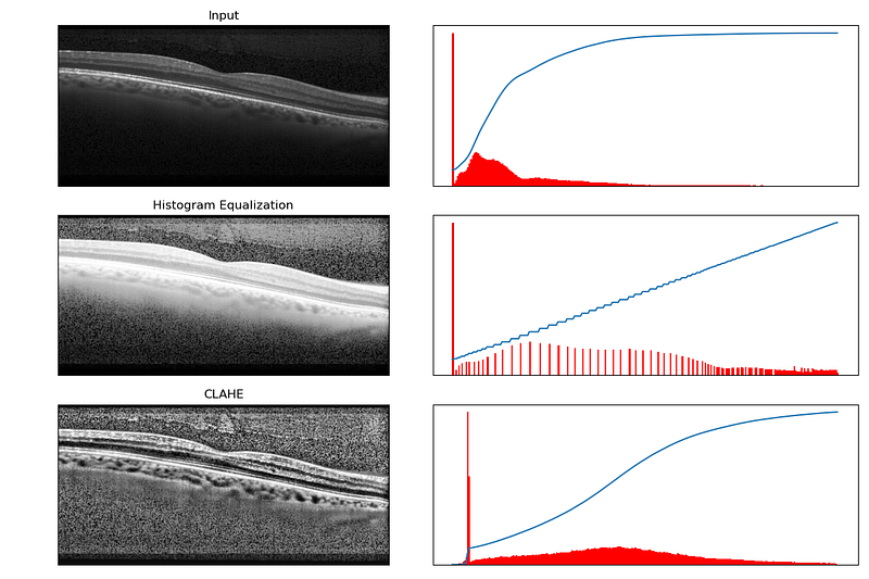
Fig. 4 and 5 show the outcomes regarding CLAHE. From Fig. 4, it is clear that CLAHE performs better compared to the HE. However, it amplifies noise components also from the retinal layer image. Fig 5 shows that the CLAHE will be more suitable in terms of visibility of different vessels and veins on the retinal surface.
The following shows the script for the above mentioned methods. Each of the method has a traceable function name, which is related to the transformation function. The implementation is mostly performed using Numpy and OpenCV in Python.
Conclusion:
In this blog, we covered the basics of image manipulation using different linear and non-linear transformation functions. These functions should be chosen based on the input image and the application. For example, inverted Gaussian function was not suitable for vessel detection but perfectly fit for the enhancement of the retinal layers image. Similarly, CLAHE was more suitable for vessel detection application compared to the layer structure enhancement.
The one of the main problem with retinal image (with layers) is noise. As it can be seen that CLAHE failed because of the noise components. Therefore, noise-removal in necessary and vital in further processing of the medical images. In the next blog, we will discuss about the different noise and noise-removal methods. Stay tuned!
Thank you very much for reading. Follow us for more Data Science & Computer Vision techniques!
The codes and example images are available at the following link:


