A Quick Guide to AUC-ROC in Machine Learning Models

A simple and robust method to compare the effectiveness of classification models should not be made complicated by too many different definitions.

One of the most common applications of Machine Learning is to classify entities into two distinct, non-overlapping categories. Over the years, several methods have been devised, ranging from very simple to more complex to almost a black-box. One common question that comes up when dealing with almost any kind of model is how to compare the performance of different methods, or different tuning of the parameters. Luckily, in the case of binary classifiers, there is a simple metric that catches the essence of the problem: it’s the Area Under the Curve (i.e. the integral) of the Receiver Operating Characteristic, hence the acronym AUC-ROC or just ROC for short.

Dealing With Your Errors

For the sake of the argument, let’s say that a tiger vs cat binary classifier identifies entities as belonging to either a true positive (tiger, accepted) or true negative (cat, rejected) case. The classifier assigns a number between 0 and 1 to each entity, if the number is larger than a given threshold (say 0.5) the entity is accepted, otherwise it’s rejected. No classifier is perfect, which means that less than 100% of the cases will be identified correctly. Most of the times, it will misidentify things for many reasons, prominently small training dataset size and intrinsic limitations of the model. In many cases, we are also trying to reject some form of “background noise” (here: cats).

Traditionally, classification errors fall in two categories which I will refer in the following as false negatives (i.e. tigers classified as cats) and false positives (i.e. cats identified as tigers). It goes without saying that identifying a cat as a tiger is nowhere near as dangerous as identifying a tiger as a cat: the two types of errors are usually not treated equally, and depending on the problem, the parameters of the classifier are optimized to minimize either type.

The ROC Curve

Having said all of this, we want to find a compact way to summarize a classifier’s performance. Intuitively, one realized easily that a given model sits at a trade-off point in the parameter space, balancing the number of true positives (TP), false positives (FP), false negatives (FN) and true negatives (TN). Once the model is trained, the only parameter we are allowed to change is the threshold of the output probability. So we scan this number from 0 to 1 and see how the performance change accordingly. However, a 4D parameter space is all but intuitive! However, it turns out that only 2 out of 4 of these numbers are actually independent, so it’s easier to combine them into something else and use that instead. Long story short, here’s a possible combination:

True Positive Rate (TPR) = TP / (TP + FN) = efficiency (εₛ) to identify the signal (also known as Recall or Sensitivity) False Positive Rate (FPR) = FP / (FP + TN) = inefficiency (ε_B) to reject background

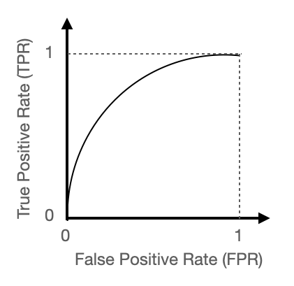
The ROC curve is nothing more than TPR vs FPR, scanned as a function of the output probability. Usually, it looks somewhat like this:

How about alternative combinations? Of course, if you take a look at the Wikipedia page , you’ll discover everything about sensitivity, recall, hit rate, or true positive rate, specificity, selectivity or true negative rate, precision or positive predictive value, negative predictive value, miss rate or false negative rate, fall-out or false positive rate, false discovery rate, false omission rate, prevalence threshold, threat score (TS) or critical success index (CSI), accuracy, balanced accuracy, Matthews correlation coefficient, Fowlkes–Mallows index, informedness or bookmaker informedness, markedness (MK) or deltaP (Δp). All of this to say that different contexts may require different definitions, but these are not necessarily as intuitive as TPR vs FPR.

Interpreting the Area Under the ROC Curve

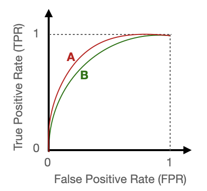
Let’s say we have two classifiers A and B. Their ROC curves look like the ones below. Which one has the better performance?

Before we answer this, we want to make some considerations. Both classifiers have an output between 0 and 1, but in general the two classifiers will have a different threshold for the same value of TFP or FPR. So, we probably want a metric that does not depend on the threshold, unless we are designing the classifier to minimize either the FP or FN type of error. Also, we want a number that is normalized, i.e. can be directly compared between the two. If I say that classifier A has a score 122 and classifier B has a score 72, it’s hard to tell…but if we know that the score is normalized between 0 and 1, then a direct comparison is easy to make.

A simple function that has this property is — guess what? — the area under the curve, i.e. the integral. Since both FPR and TPR are between 0 and 1, the area can’t be smaller than 0 and can’t be larger than 1, either.

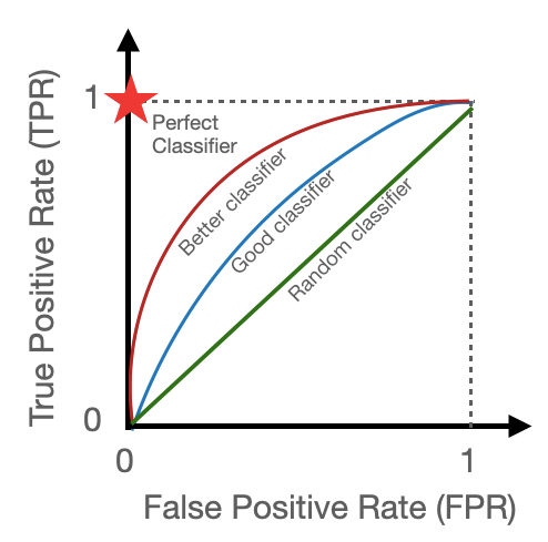
Since a picture is worth a thousand words, here’s a picture showing how to spot the performance of different classifiers just by looking at the AUC-ROC:

In practice, you will probably end up using a function from some pre-defined library, such as that from scikit-learn. The function needs the true labels in order to compare the result of the threshold scan against the ground truth.

from sklearn.datasets import load_breast_cancer
from sklearn.linear_model import LogisticRegression
from sklearn.metrics import roc_auc_score
X, y = load_breast_cancer(return_X_y=True)
clf = LogisticRegression(solver="liblinear", random_state=0).fit(X, y)
roc_auc_score(y, clf.predict_proba(X)[:, 1])
0.99

Does this work for multiclass as well? Yes indeed: just plot one class vs the others.

Conclusions

Calculating the Area under the Receiver Operating Characteristic curve is the most intuitive tool to compare the effectiveness of different classifiers. While there are some known limitations, e.g. when you want to minimize certain types of error, this is probably the most effective way to convince anyone that a classifier is doing its job better than randomly picking up the answer. As a word of caution, comparing different classifiers, especially belonging to different classes, usually requires much more carefully thinking, as for example the dataset needed to train a Decision Tree may be smaller than what’s needed to train a Deep Neural Network, but their efficiency in some particular edge cases may be subtle and hard to spot just by looking at a single number such as AUC-ROC.