
A Primer to Auto Insurance Pricing for Data Scientists

The skillsets of Data scientists can have a wide range of applications. If you are interested in this article, I may guess you are a data scientist who has a wide range of interests and wants to see how your data science skill can apply to the development of an auto insurance pricing model. Does the insurance industry use data science? Yes. The term “insurance” may not sound as rosy as “tech”, but the operations of an insurance business rely on a large body of data science techniques as well as information technology.
An insurance contract is a financial obligation. It has no tangible product. If you list a product on Amazon.com for sale, you know your costs and you add your markup to list your price. The cost is known before you sell the product. But an insurance company does not know its cost at the beginning of a year. So an insurance company has to employ statistical methods to predict the cost. That’s the fundamental difference between an insurance company and other businesses that sell physical goods.
Today data scientists are in huge demand in the insurance industry to model and estimate costs. The modeling of insurance pricing is at the core of the insurance industry. And now with the advance in data science, more data scientists and engineers continue to contribute to insurance pricing.
This article assumes you have some regression background. It is not an article to explain what regression is. It intends to share with you the development of an auto-pricing model. It starts with the coverages of auto insurance so you know what the models are built for. It then describes the data preparation, modeling building, to the relativities. This article does not assume you have an insurance background and will explain any insurance jargon if ever mentioned. In the end, I include both Python and R examples and further references.
(A) Different Premiums to Reflect Different Risks
If a reckless driver is charged the same premium, say $1,000, as a conservative driver, what will happen? The reckless driver will feel the insurance charge is cheap, but the conservative driver feels it is too expensive. The reckless driver will buy your auto insurance but the conservative driver won’t. As a result, your book of business will only have reckless drivers who are likely to demand higher-than-expected financial obligations. This is called adverse selection. What can an insurer do? The insurer should charge differential rates based on the risk characteristics of drivers. For example, charging the reckless driver $1,500 and the conservative driver $500 (the average is still $1,000). Also, the insurer should develop a sound procedure to verify any misrepresentation of information.
For years insurance companies have been trying to improve their rate-making scheme, develop new methods, and to determine a reasonable risk-based rate structure and appropriately differentiate between the policyholders. The key to providing the customer-specific differential rating scheme is good data science modeling as well as good data: predicting the expected claim level for each customer as a function of the variables. This problem is challenging. Also, with the coming of telematics, the pricing work will be even more demanding. See “Telematics in Auto Insurance”.
(B) What Does Auto Insurance Cover?
Automobile accidents can cause great financial stress. Financial loss may include property damage, medical bills, and legal costs if a lawsuit arises. Anyone who owns a car should purchase auto insurance so that these important financial protections are provided. Most states either require the owner of a vehicle to purchase auto insurance.
(B.1) Bodily Injury (BI) Liability Coverage
Most auto liability insurance policies contain three major parts:
- Bodily injury: If you cause an accident and other people are injured due to your negligence, this insurance protects you against their claims for damages, such as medical expenses, lost wages, and financial compensation for their pain and suffering. This coverage does not protect you or your car. This is the biggest expense to an insurance company if compared with the items below.
- Property damage: This coverage pays for any damage you cause to the property of others, such as another vehicle, fence, or tree caused by a collision.
- Uninsured motorist: This coverage pays if you are injured by a driver (e.g. hit-and-run) who does not have auto liability insurance. In other words, you buy the coverage that the other driver should have purchased but did not. Underinsured motorist coverage applies when the other driver is at fault and whose limits of liability are lower than the damages you sustained.
Some states have no-fault laws — meaning there is no need to determine who is at fault to receive payment for injury claims. Each party would seek recovery from his/her insurer instead of bringing a lawsuit. No fault does not eliminate the risk of you being sued. However, no-fault laws do place restrictions on when a suit can be brought forward. There are two typical types of coverage provided under a no-fault system. These coverages are Personal Injury Protection (PIP) and Residual Bodily Injury Liability Coverage.
No-fault laws usually have certain thresholds that, if exceeded, open the possibility of a suit. These thresholds can be based on a specific dollar amount, clearly defined injuries, and/or a death resulting from an accident.
- Personal Injury Protection (PIP): This covers any other person riding in your car a minimum amount per person for injury regardless of fault. Coverage typically includes medical expenses, rehabilitation expenses, work loss benefits (loss wages), funeral expenses, and survivor’s loss benefits.
- Residual Bodily Injury Liability Coverage: This protects you and anyone driving your car with your permission if you are sued because of injuries caused to others.
(B.2) Physical Damage (PD) Coverage for the Car
There are two types of coverages:
- Collision Coverage: This covers physical damage to your car as a result of your auto colliding with an object, such as another car or a tree.
- Comprehensive Coverage pays: This covers damage to your auto from almost all other losses other than collision. Covered losses under comprehensive coverage include the following: theft, fire, vandalism, weather-related losses such as hail, water (flood), falling objects, damage caused by a bird or animal, and glass breakage.
The above just describes two major types (BI and PD). There are additional coverages such as Medical Payment Coverage, Rental reimbursement coverage, Emergency Roadside Service coverage, or Windshield coverage. We need to understand the coverages to develop auto-pricing models. In your auto premiums, you may see three items like Bodily injury, Physical damage, and comprehensive. The premium of each category is determined by a model or models.
(C) The Main Output of a Loss Cost Model Is the Rate Relativities
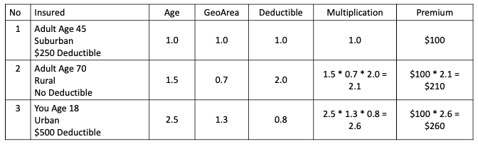
Table 1 shows hypothetical relativities. There are three individuals. The values in the table are called the “relativities”. Individual 2 is a senior adult aged 70. From experience, a senior adult is 1.5 times “relative” risky compared to Individual 1 who is mid-age 45. All the relativities are multiplicative. If the premium for Individual 1 is $100 the base rate, then the premium for Individuals 2 and 3 should be $210 and $260 respectively. At the end of the article, I show an example of the rate relativities.
(D) Prepare the Data
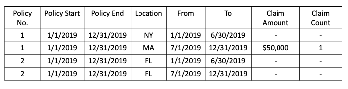
Split the policy at the desired level of temporal granularity such as monthly, quarterly, or half-yearly. Usually, all motor insurance policies are of a one-year duration. There will be policyholders moving from one location to another during a policy year. To capture the location difference, Table 2 is a special case that presents the data on the half-year level. Policyholder 1 lived in New York in the first half of the policy year and then moved to Massachusetts in the second half of the policy year.
There are a few things to remember. First, the claim amount below a certain threshold should be removed from modeling because such claims could be below the deductible limit.
(E) Frequency-Severity (F-S) Modeling: Standard Way
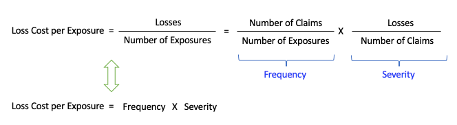
Actuaries use the terms Frequency and Severity. Let’s give a formal definition. Frequency is the likelihood that a loss will occur. For example, if there are 10,000 car accidental claims out of 1,000,000 insured cars. The frequency is 10,000/1,000,000 = 1%. Frequency is usually a low number. in this case 990,000 cars report no accident. Severity is the average size of a claim. Suppose the total loss amount of the 10,000 cars is $1,000,000,000, the severity is $1,000,000,000/10,000 = $100,000. The definitions are written below:
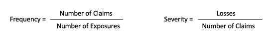
Because there are 1 million cars insured and the total loss amount is $1 billion, the Loss Cost per insured car is $1 billion / $1 million = $1,000, which is also the frequency multiplying severity 1% x $100,000 = $1,000. Why do I elaborate on the relationship between frequency and severity and loss cost? It is because loss cost per exposure is frequency multiplying severity, see the relationship below.
Actuaries have found empirically that frequency follows an over-dispersed Poisson distribution and severity follows a Gamma distribution. We build a frequency model and a severity model. We then multiply the predictions of the two to get the predicted loss cost per exposure.
(F) Frequency-Severity (F-S) Modeling: More Sophisticated Way
Extreme values are difficult to model. If there exists a wide range of extreme values, the above approach may be too simplistic. A practical solution is to model them separately and then add them together. Let’s modify the formula to cap the severity, and model the probability of excess claim and the size of the excess severity separately:
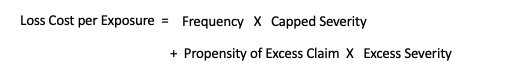
And the distributions are assumed for the above terms:
- Frequency: Over-dispersed Poisson distribution
- Capped Severity: Gamma distribution
- The propensity of excess claim: Binomial distribution
- Excess Severity: Gamma distribution
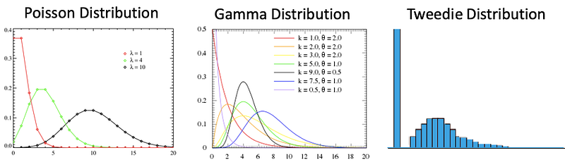
The frequency measures the count of an accident. In a year most cars report zero accidents. The Poisson distribution has the nice property that there are more zeros as shown in the graph below. Of the cars involved in accidents, a small percentage will have severe damage. If you plot the count statistic by damage dollars, which is the histogram, you will see a long tail to the high-dollar values. The Gamma distribution is a nice choice to model a long-tail distribution.
(G) Verify the F-S Distributions with the Actual Data
The frequency model uses the claim count “number of claims” as the target variable: Let’s assume you have 1,000,000 auto policy-year records. Assume there are 80% zero claims, 18% one claims, 1.8% two claims, and 0.2% more than two claims. You can cap the “more than two claims” to be two. So your target variable has three values: 0, 1, and 2. The frequency model is developed on 1,000,000 datasets.
The severity model uses only the claims that the claim amount is more than $0. Of the above 1,000,000 records, only 20% have accidents. So the severity model is developed on the 200,000 records. Once the severity model is developed, it is then applied to score the entire 1,000,000 records. Therefore every record will have a frequency score and a severity score. Multiplying the two scores you get the loss cost dollars.
Verify the distributions: You will perform formal tests to see the Poisson and Gamma distribution.
(H) Loss-Cost (LC) Modeling using the Tweedie Distribution
Statistically, a Poisson distribution compounding the Gamma distribution becomes the Tweedie distribution, as shown in the above graph. The Tweedie distribution is a special case of exponential dispersion models. The distribution has more count at zero then follows by a long-tail curve. In other words, it has a mixture of zeros and non-negative continuous data. This particular property makes it suitable for modeling frequency and severity in one step. The Tweedie can be used in other industries as long as the histogram of your target variable shows a spike at zeros and a long tail in the non-zeros.
(I) Which One? F-S or LC?
Shall you use the F-S approach to build two models and then multiply the predictions together, or the LS approach which involves one modeling step? Either method has its advantages. The F-S modeling approach can provide more insights because frequency and severity could have different patterns. Often the frequency model and the severity model show different variables (and the severity model has fewer variables). In contrast, the LC approach usually shows better goodness of fit than the F-S approach because it builds one model.
(J) The Best Modeling Practices — F-S Refit to LC
It appears the F-S and the LC approach are all employed by data scientists. This also gives them the chance to double-check the parameter estimates generated based on the F-S approach. Refitting the actual loss cost seems a popular approach:
- Build the frequency and severity models separately. Generate frequency score and severity score, then get LC score = (Frequency Score) x (Severity Score).
- Use the above LC score to refit the actual LC. This step can generate LC Relativities.
(K) Things to Consider for Relativities
In setting rate relativities, we have to inspect from an actuarial, operational, social, and legal perspective.
Actuarial Perspective:
- Fairly discriminatory: Rate relativities should reflect accurately the risks to reduce adverse selection.
- Homogeneity: Members of the same class should be homogeneous, i.e., with similar expected costs.
- Credibility: Each class group should be large enough to measure costs with sufficient accuracy.
- Stability: The differences in the estimated cost between groups should be relatively stable over time. This does not mean they will be the same over time.
Operational perspective:
- Efficiency: The operational expense should be the most efficient. If there is an additional cost in obtaining & verifying information, it should be justifiable.
Social perspective:
- The privacy should be protected.
- Affordability: If rates are too high, they can be capped for certain groups so they to afford the minimum insurance needed.
Legal perspective:
- The choice of rating variable may be prohibited by law, including gender, race, or income.
(L) Prepare the Pure Premium Outcome
Suppose you have developed the models for each peril and have scored all the records. How do you derive the pure premium? To reflect the likely future mix of business, you should select the dataset that can reflect the mix of future business. You can do the following:
- Loss Cost = Frequency score x Severity score
- Add up the loss costs of the perils. For example, if the predicted loss costs for BI and PD are $1,000 and $500 for a policyholder, the pure premium is $1,500.
(M) Python Examples
Click here for the Python code snippet that shows you how to develop the loss-cost models with Poisson, Gamma, and Tweedie distributions. The data features include typical features such as driver age, vehicle age, vehicle power, etc. Each record corresponds to an insurance policy, i.e. a contract within an insurance company and an individual (policyholder).
- It first models the number of claims with a Poisson distribution.
- It models the severity as a Gamma distribution.
- It then multiplies the predictions of both to get the total claim amount.
(N) R Code Examples
This example provides the R code for the models in the book “Non-life Insurance Pricing with Generalized Linear Models”. The code below is just a reproduction of the book example. I will reference what was described in the above content in the code. This way you can see how it is done.
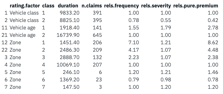
First, the frequency model regresses the claim count (antskad) on the rating variables (“premiekl”, “moptva”, “zon”), and takes “dur” as the offset. The offset is log(dur) because our link function is log.
The coefficients from the frequency model are converted to the relativities.
Second, because the Gamma distribution is used for the severity model, the zero values are removed. This is done by table.1.2[table.1.2$medskad > 0, ]. Then the coefficients from the severity model are converted to the relativities.
Third, with the frequency and severity relativities, the pure premium can be derived by multiplying both:
Conclusion
I hope this article gives you a better understanding of this topic. I suggest you read the following articles for a comprehensive review:


