Early Stopping in Practice: an example with Keras and TensorFlow 2.0

A step to step tutorial to add and customize Early Stopping

In this article, we will focus on adding and customizing Early Stopping in our machine learning model and look at an example of how we do this in practice with Keras and TensorFlow 2.0.

Introduction to Early Stopping

In machine learning, early stopping is one of the most widely used regularization techniques to combat the overfitting issue.

Early Stopping monitors the performance of the model for every epoch on a held-out validation set during the training, and terminate the training conditional on the validation performance.

From Hands-on ML [1]

Early Stopping is a very different way to regularize the machine learning model. The way it does is to stop training as soon as the validation error reaches a minimum. The figure below shows a model being trained.

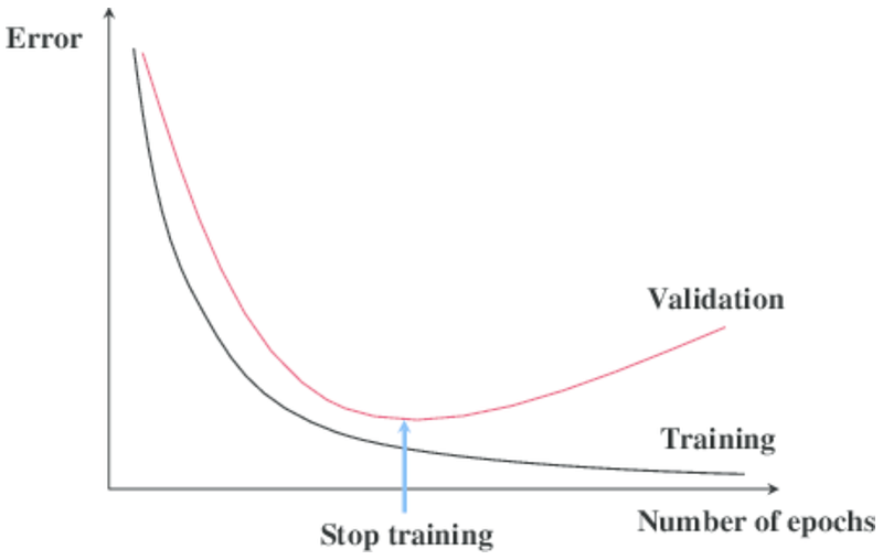
As the epochs go by, the algorithm leans and its error on the training set naturally goes down, and so does its error on the validation set. However, after a while, the validation error stops decreasing and actually starts to go back up. This indicates that the model has started to overfit the training data. With Early Stopping, you just stop training as soon as the validation error reaches the minimum.

It is such a simple and efficient regularization technique that Geoffrey Hinton called it a “beautiful free lunch.” [1].

With Stochastic and Mini-batch Gradient Descent

With Stochastic and Mini-batch Gradient Descent, the curves are not so smooth, and it may be hard to know whether you have reached the minimum or not. One solution is to stop only after the validation error has been above the minimum for some time (when you are confident that the model will not do any better), then roll back the model parameters to the point where the validation error was at a minimum.

In the following article, we are going to add and customize Early Stopping in our machine learning model.

Environment setups and dataset preparation

We will be using the same dataset as we did in the model regularization and batch normalization. You can skip this chapter if you are already familiar with it.

In order to run this tutorial, you need to install

TensorFlow 2, numpy, pandas, sklean, matplotlib

They can all be installed directly vis PyPI and I strongly recommend to create a new Virtual Environment. For a tutorial on creating a Python virtual environment

Source code

This is a step by step tutorial and all instructions are in this article. For source code, please check out my Github machine learning repo.

Dataset preparation

This tutorial uses the Anderson Iris flower (iris) dataset for demonstration. The dataset contains a set of 150 records under five attributes: sepal length, sepal width, petal length, petal width, and class (known as target from sklearn datasets).

First, let’s import the libraries and obtain iris dataset from scikit-learn library. You can also download it from the UCI Iris dataset.

import tensorflow as tf
import pandas as pd
import numpy as np
import matplotlib.pyplot as plt
from sklearn.datasets import load_iris
from sklearn.model_selection import train_test_split

iris = load_iris()

For the purpose of exploring data, let’s load data into a DataFrame

# Load data into a DataFrame
df = pd.DataFrame(iris.data, columns=iris.feature_names)
# Convert datatype to float
df = df.astype(float)
# append "target" and name it "label"
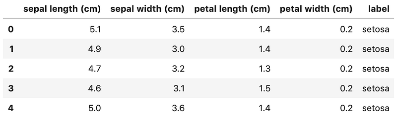
df['label'] = iris.target
# Use string label instead
df['label'] = df.label.replace(dict(enumerate(iris.target_names)))

And the df should look like below:

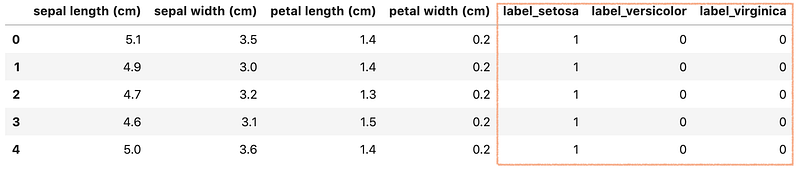
We notice the label column is a categorical feature and will need to convert it to one-hot encoding. Otherwise, our machine learning algorithm won’t be able to directly take in that as input.

# label -> one-hot encoding
label = pd.get_dummies(df['label'], prefix='label')
df = pd.concat([df, label], axis=1)
# drop old label
df.drop(['label'], axis=1, inplace=True)

Now, the df should look like:

Next, let’s create X and y. Keras and TensorFlow 2.0 only take in Numpy array as inputs, so we will have to convert DataFrame back to Numpy array.

# Creating X and yX = df[['sepal length (cm)', 'sepal width (cm)', 'petal length (cm)', 'petal width (cm)']]
# Convert DataFrame into np array
X = np.asarray(X)y = df[['label_setosa', 'label_versicolor', 'label_virginica']]
# Convert DataFrame into np array
y = np.asarray(y)

Finally, let’s split the dataset into a training set (80%)and a test set (20%) using train_test_split() from sklearn library.

X_train, X_test, y_train, y_test = train_test_split(
  X,
  y,
  test_size=0.20
)

Great! our data is ready for building a Machine Learning model.

Build a neural network

There are 3 ways to create a machine learning model with Keras and TensorFlow 2.0. Since we are building a simple fully connected neural network and for simplicity, let’s use the easiest way: Sequential Model with Sequential().

Let’s go ahead and create a function called create_model() to return a Sequential model.

from tensorflow.keras.models import Sequential
from tensorflow.keras.layers import Dense

def create_model(): 
    model = Sequential([
        Dense(64, activation='relu', input_shape=(4,)),
        Dense(128, activation='relu'),
        Dense(128, activation='relu'),
        Dense(128, activation='relu'),
        Dense(64, activation='relu'),
        Dense(64, activation='relu'),
        Dense(64, activation='relu'),
        Dense(3, activation='softmax')
    ])
    return model

Our model has the following specifications:

The first layer (also known as the input layer) has the input_shape to set the input size (4,)
The input layer has 64 units, followed by 3 dense layers, each with 128 units. Then there are further 3 dense layers, each with 64 units. All these layers use the ReLU activation function.
The output Dense layer has 3 units and the softmax activation function.

Compile and train the model

In order to train a model, we first have to configure our model using compile() and pass the following arguments:

Use Adam (adam) optimization algorithm as the optimizer
Use categorical cross-entropy loss function (categorical_crossentropy) for our multiple-class classification problem
For simplicity, use accuracy as our evaluation metrics to evaluate the model during training and testing.

model.compile(
    optimizer='adam', 
    loss='categorical_crossentropy', 
    metrics=['accuracy']
)

After that, we can call model.fit() to fit our model to the training data.

history = model.fit(
    X_train, 
    y_train, 
    epochs=200, 
    validation_split=0.25, 
    batch_size=40, 
    verbose=2
)

If all runs smoothly, we should get an output like below

Train on 84 samples, validate on 28 samples
Epoch 1/200
84/84 - 1s - loss: 1.0901 - accuracy: 0.3214 - val_loss: 1.0210 - val_accuracy: 0.7143
Epoch 2/200
84/84 - 0s - loss: 1.0163 - accuracy: 0.6905 - val_loss: 0.9427 - val_accuracy: 0.7143
......
Epoch 200/200
84/84 - 0s - loss: 0.5269 - accuracy: 0.8690 - val_loss: 0.4781 - val_accuracy: 0.8929

Plot the learning curves

Finally, let’s plot the loss vs. epochs graph on the training and validation sets.

It is preferable to create a small function for plotting metrics. Let’s go ahead and create a function plot_metric().

%matplotlib inline
%config InlineBackend.figure_format = 'svg'def

plot_metric(history, metric):
    train_metrics = history.history[metric]
    val_metrics = history.history['val_'+metric]
    epochs = range(1, len(train_metrics) + 1)
    plt.plot(epochs, train_metrics)
    plt.plot(epochs, val_metrics)
    plt.title('Training and validation '+ metric)
    plt.xlabel("Epochs")
    plt.ylabel(metric)
    plt.legend(["train_"+metric, 'val_'+metric])
    plt.show()

By running plot_metric(history, 'loss') to get a picture of loss progress.

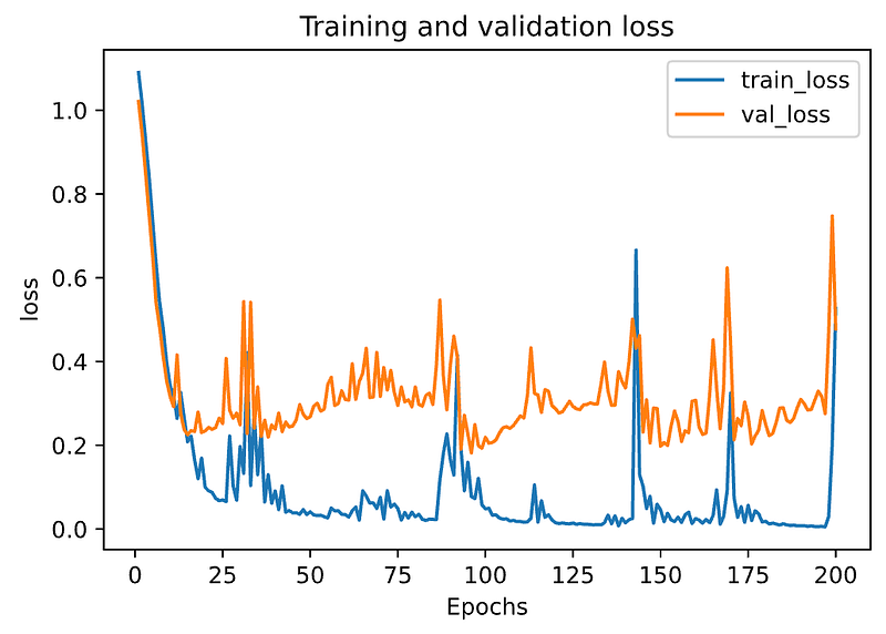
From the above graph, we can see that the model has overfitted the training data, so it outperforms the validation set.

Adding Early Stopping

The Keras module contains a built-in callback designed for Early Stopping [2].

First, let’s import EarlyStopping callback and create an early stopping object early_stopping .

from tensorflow.keras.callbacks import EarlyStopping

early_stopping = EarlyStopping()

EarlyStopping() has a few options and by default:

monitor='val_loss': to use validation loss as performance measure to terminate the training.
patience=0: is the number of epochs with no improvement. The value 0 means the training is terminated as soon as the performance measure gets worse from one epoch to the next.

Next, we just need to pass the callback object to model.fit() method.

history = model.fit(
    X_train, 
    y_train, 
    epochs=200, 
    validation_split=0.25, 
    batch_size=40, 
    verbose=2,
    callbacks=[early_stopping]
)

You can see that early_stopping get passed in a list to the callbacks argument. It is a list because in practice we might be passing a number of callbacks for performing different tasks, for example debugging and learning rate scheduler.

By executing the statement, you should get an output like below:

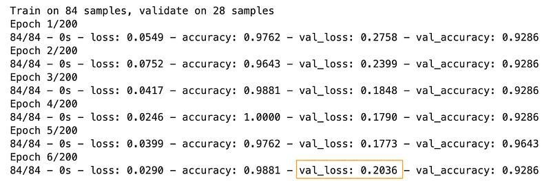
Note: your output can be different due to the different weight initialization.

The training gets terminated at Epoch 6 due to the increase of val_loss value and that is exactly the conditions monitor='val_loss' and patience=0.

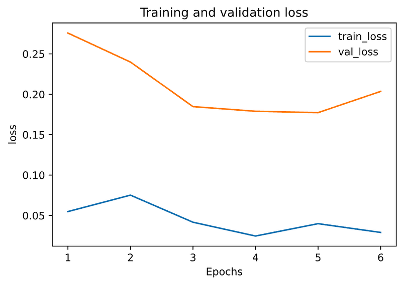
It’s often more convenient to look at a plot, let’s run plot_metric(history, 'loss') to get a clear picture. In the below graph, validation loss is shown in orange and it’s clear that validation error increases at Epoch 6.

Customizing Early Stopping

Apart from the options monitor and patience we mentioned early, the other 2 options min_delta and mode are likely to be used quite often.

monitor='val_loss': to use validation loss as performance measure to terminate the training.
patience=0: is the number of epochs with no improvement. The value 0 means the training is terminated as soon as the performance measure gets worse from one epoch to the next.
min_delta: Minimum change in the monitored quantity to qualify as an improvement, i.e. an absolute change of less than min_delta, will count as no improvement.
mode='auto': Should be one of auto, min or max. In 'min' mode, training will stop when the quantity monitored has stopped decreasing; in 'max' mode it will stop when the quantity monitored has stopped increasing; in 'auto' mode, the direction is automatically inferred from the name of the monitored quantity.

And here is an example of a customized early stopping:

custom_early_stopping = EarlyStopping(
    monitor='val_accuracy', 
    patience=8, 
    min_delta=0.001, 
    mode='max'
)

monitor='val_accuracy' to use validation accuracy as performance measure to terminate the training. patience=8 means the training is terminated as soon as 8 epochs with no improvement. min_delta=0.001 means the validation accuracy has to improve by at least 0.001 for it to count as an improvement. mode='max' means it will stop when the quantity monitored has stopped increasing.

Let’s go ahead and run it with the customized early stopping.

history = model.fit(
    X_train, 
    y_train, 
    epochs=200, 
    validation_split=0.25, 
    batch_size=40, 
    verbose=2,
    callbacks=[custom_early_stopping]
)

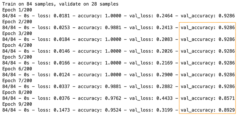
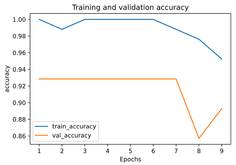
This time, the training gets terminated at Epoch 9 as there are 8 epochs with no improvement on validation accuracy (It has to be ≥ 0.001 to count as an improvement). For a clear picture, let’s look at a plot representation of accuracy by running plot_metric(history, 'accuracy'). In the below graph, validation accuracy is shown in orange and it’s clear that validation accuracy hasn’t got any improvement.

That’s it

Thanks for reading.

Please checkout the notebook on my Github for the source code.

Stay tuned if you are interested in the practical aspect of machine learning.

References

[1] Hands-on Machine Learning with scikit-learn, keras, and tensorflow: concepts, tools, and techniques to build intelligent system
[2] Keras Official Documentation for Early Stopping