
A Practical Guide to ARIMA Models using PyCaret — Part 3
Understanding the Difference Term

📚 Introduction
In the previous article in this series, we saw the impact of the trend term on the output of an ARIMA model. This article will look at the “difference” term “d” and see how this is modeled and what it represents.
📖 Suggested Previous Reads
The previous articles in this series can be found below. I would recommend that readers go through them first before continuing with this article. This article builds upon the concepts described in the previous ones as well as reuses some work done in it.
A Practical Guide to ARIMA Models using PyCaret — Part 1
A Practical Guide to ARIMA Models using PyCaret — Part 2
1️⃣ “Differencing — d” Overview in ARIMA Models
At a very high level, differencing means that the value of a time series at any given point in time depends on the value(s) at a previous point in time. A difference “d = 1” means that the value at any point in time depends on the previous point in time (given by equation 1). The epsilon term represents the noise term which can not be modeled.

Important Side Note: The process that generates a time series using equation 1 is also called a “Random Walk”. Most stock data follows this pattern. If you look closely, you will realize that when this is modeled correctly, the best prediction of the future point is the same as the last known point. Hence, stock price models using traditional approaches like ARIMA do not produce “useful” models. Do we really need a model to tell us that tomorrow’s stock price will be the same as today’s stock price?
2️⃣️ Understanding the Difference Term using PyCaret
👉 Step 1: Setup PyCaret Time Series Experiment
In order to understand this concept better, we will use a random walk dataset from pycaret playground. Details can be found in the Jupyter notebook for this article (available at the end of the article).
#### Get data from data playground ----
y = get_data("1", folder="time_series/random_walk")
exp = TimeSeriesExperiment()
exp.setup(data=y, seasonal_period=1, fh=30, session_id=42)exp.plot_model()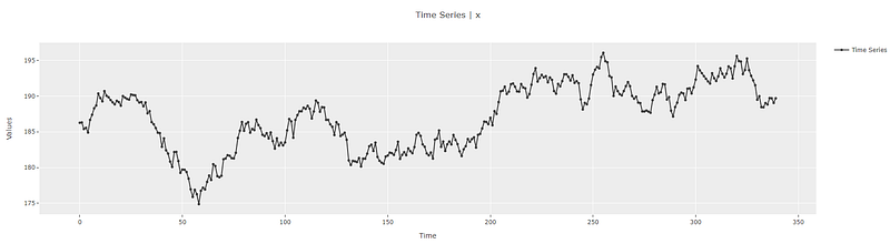
👉 Step 2: Perform EDA
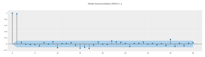
A classical way to diagnose whether a time series has been generated using a random walk process is to look at the ACF and PACF plots. ACF plots will show extended auto-correlations [1]. PACF plots should show a peak at lag = 1 and the peak should be very close to 1 in magnitude. All other lags will be insignificant. You can think about the PACF magnitude as the coefficient of the lagged value y(t-1) in equation 1. I will write more about this in another article.
exp.plot_model(plot="acf")
exp.plot_model(plot="pacf")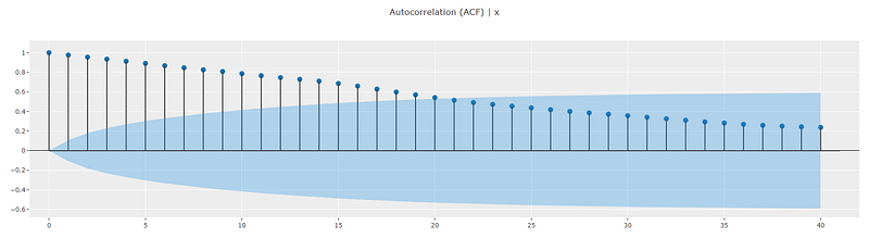
👉 Step 3: Theoretical Calculations
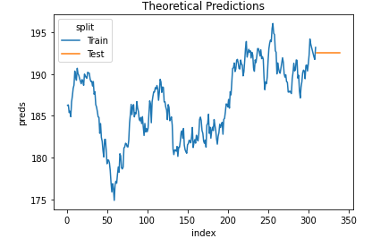
For a random walk model, we can use equation 1 to guide us in calculating theoretical values. Essentially, the next time point is predicted to be the last “known” time point. For in-sample predictions (i.e. predictions on the training dataset), this will change at every point in time since the last known point at t = 1 is not the same as the last “known” point at t = 10 (assuming both t=1 and t=10 are in-sample).
For the out-of-sample predictions (i.e. predictions in the unknown cross-validation/test dataset), the best future prediction will be the last known data point. This remains the same no matter how far we predict the future. This is an important distinction between in-sample and out-of-sample predictions for a random walk.
👉 Step 4: Build the Model with PyCaret
#### Random Walk Model (without trend) ----
model3a = exp.create_model(
    "arima",
    order=(0, 1, 0),
    seasonal_order=(0, 0, 0, 0),
    trend="n"
)
👉 Step 5: Analyze the Results
We will reuse the same helper functions that we created in the previous articles to analyze the results.
summarize_model(model3a)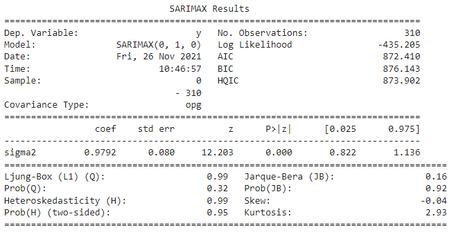
The statistical summary shows that the created model is a SARIMAX(0,1,0) model which matches our desire to build a model with d=1. The residual sigma2 (unexplained variance) is 0.9720 and representative of the epsilon term in equation 1.
get_residual_properties(model3a)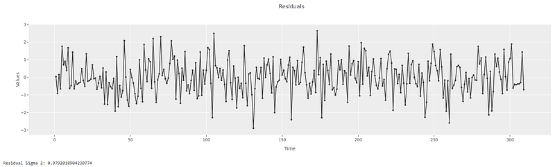
Looking at the model residuals, we can see that residuals indeed have a variance of 0.9720 which matches with the statistical summary. Next, let’s plot the predictions and compare to our theoretical framework.
plot_predictions(model3a)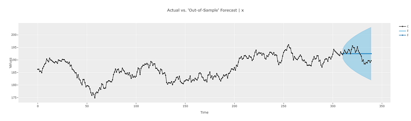
The out-of-sample predictions match our theoretical calculations. i.e. the predictions are the same as the last known data point (in this case the value at point 309). The ability to zoom into the interactive plots in pycaret makes it easy to analyze the results and gain better intuition into the working of the model.
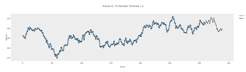
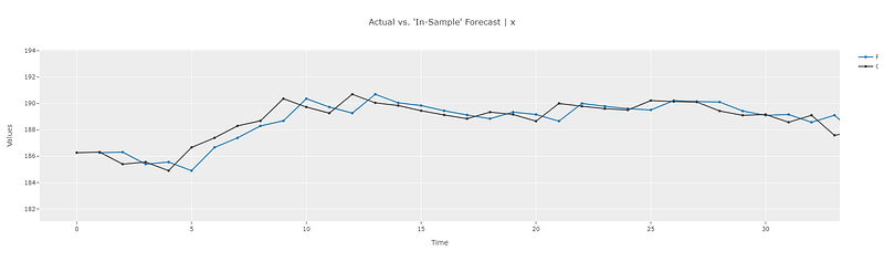
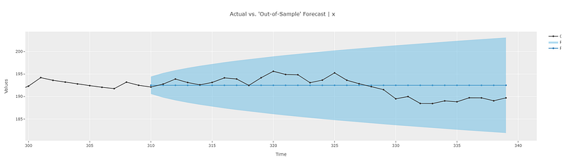
Similarly, we can observe the in-sample predictions as well. Zooming into the plot shows that the prediction at any given point in time is the same as the last known point. And since the last known data point changes from one time point to the next, the in-sample prediction also changes from one point to the next. This also matches with our theoretical calculations.
👉 Step 6: Checking the Model Fit
This is also a good time to introduce the concept of “model fit”. Checking the model fit essentially means checking to see if the model has captured all the “information” from the time series or not. This is true when the model residuals do not have any trend, seasonality, or auto-correlations, i.e. the residuals are “white noise”. pycaret provides a very handy feature to check model fit. We can check the white noise characteristics of a model’s residuals by passing a model to the check_stats method/function as follows.
exp.check_stats(model3a, test="white_noise")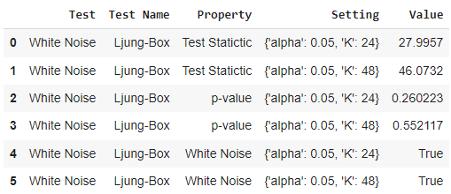
Lines 4 and 5 confirm that the residuals are indeed white noise and hence the model has captured the information from the time series well.
🚀 Conclusion
Hopefully, this simple model has laid a good foundation for us to understand the inner workings of the “difference term — d” in an ARIMA model. In the next article, we see how we can combine the “difference” term “d” with the “trend” component that we learned about in the previous article in this series. Until then, if you would like to connect with me on my social channels (I post about Time Series Analysis frequently), you can find me below. That’s it for now. Happy forecasting!
📘 GitHub
Loved the article? Become a Medium member to continue learning without limits. I’ll receive a portion of your membership fee if you use the following link, with no extra cost to you.
📗 Resources
- Jupyter Notebook containing the code for this article
📚 References
[1] Time Series Exploratory Analysis | Autocorrelation Function (ACF)


