A Practical Guide for Outlier Detection — and Implementation in Python

We have outlier values when essentially some data points are significantly different from their peers or out of context. What can you do then to ensure that these outlier values do not affect later data analysis and machine learning? In this article I will briefly review the basic methods and Python implementation.

The Basics

1) What are outliers?

Let’s start with the basics: what is an outlier in a data series?

In short, outliers in a dataset refer to data points that significantly differ from the majority of the other data points. Outliers can have many causes, such as:

• Measurement or input error
• Data corruption
• Sensor lack of calibration
• True outlier observation

2) Effects of outliers

Outliers can substantially affect statistical analyses and machine learning models:

• It increases the error variance and reduces the power of statistical tests, for example it can skew the mean and standard deviation
• They can bias or influence estimates, mislead interpretations of correlations or patterns
• It can distort the results of subsequent data processing steps, such as the values of a moving average filter
• Learning and accuracy of machine learning models can be negatively affected (Linear regression or Distance-based methods)

Let’s look at some examples of different cases:

The simplest way to test this is to plot each variable on a scatterplot. In some cases it is clear or suspected that there are outlier values in the data series. In the sample data below, we can see that there are 1 extreme value on the top that are likely an outlier.

In other cases, however, it is not always so clear which values are outliers. Consider the lineplot example below, which shows the measured values of a sensor. It can be seen that outliers with varying amplitude occur continuously, but it would be difficult to determine at first which values are still normal and which are outliers.

As can be seen from the above, it is important to perform several tests to accurately separate outliers from our data. Let’s look at how this can be done.

3) Types of outliers

Outlier can be of two types:

• univariate
• multivariate

In definition: Univariate outliers are data points that are extreme in the context of a single variable, while Multivariate outliers are observations that are extreme not in just one variable but in relationships among multiple variables.

For example: In a dataset containing both age and income, a person with an extremely high or low age compared to the majority of persons’ ages would be considered a univariate outlier.

However, when age and income are compared to each other, an extremely high value compared to others might be considered a multivariate outlier.

It is important to see the difference between them, as different methods can be used to detect them.

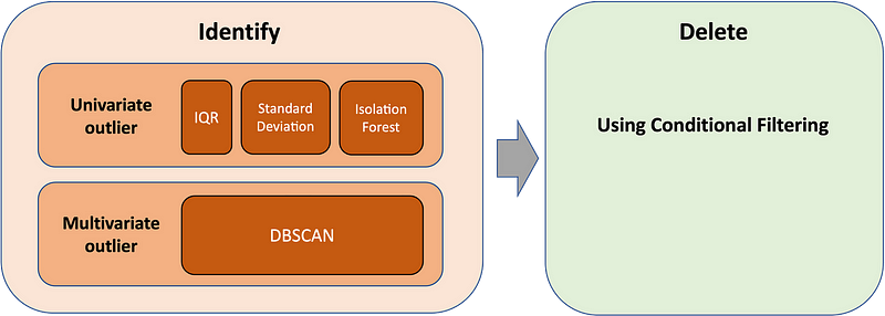
What you can do?

The essence of dealing with outliers will be as follows:

1. Identify
2. Delete

The more difficult task will be to identify and separate the values. The basic principle is to define a boundary line or area, and the data points that fall within this boundary are considered normal values. The outliers will be those data points that fall outside the boundary.

The deletion of outlier values after identification can be easily achieved by a conditional filter.

First, let’s look at what methods are available for identification.

1) Identify Univariate Outliers

For the univariate type, lets look at the most common and easy-to-implement methods:

a) Interquartile Range (IQR) Method

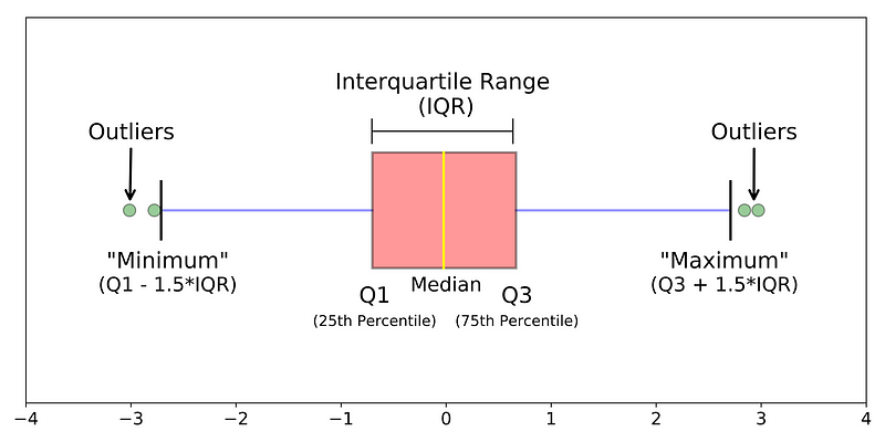
The concept of the IQR is used to build the boxplot graphs. IQR is a concept in statistics that is used to measure the statistical dispersion and data variability by dividing the dataset into quartiles.

In simple words, any dataset or any set of observations is divided into four defined intervals based upon the values of the data and how they compare to the entire dataset. A quartile is what divides the data into three points and four intervals.

It is the difference between the third quartile and the first quartile (IQR = Q3 -Q1). Outliers in this case are defined as the observations that are below (Q1 − 1.5x IQR) or boxplot lower whisker or above (Q3 + 1.5x IQR) or boxplot upper whisker. It can be visually represented by the below boxplot.

We have thus defined the boundary lines separating the normal and outlier values. In Python, we can easily calculate their values:

Q1 = np.percentile('dataset', 25)
Q3 = np.percentile('dataset', 75)
IQR = Q3 - Q1

upper_limit = Q3+1.5*IQR
lower_limit = Q1-1.5*IQR

You can then use the following condition to write the outlier values to the ‘outlier’ vector, after which they can be deleted:

outliers = 'dataset'[('dataset' > upper_limit) | ('dataset' < lower_limit)]

b) Standard Deviation

Standard deviation is a metric of variance that how much the individual data points are spread out from the mean. If a data distribution is approximately normal, then about 68.26% of the data values lie within one standard deviation of the mean and about 95.44% are within two standard deviations, and about 99.72% lie within three standard deviation border. This is visualised in the figure below:

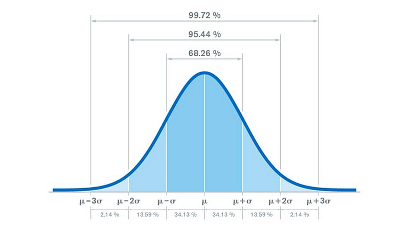
This suggests that there are very few data outside the three standard deviation limit and that their values are very different from the mean. In conclusion, we can consider this as the border between normal and outlier data. (In some cases, when data collection suggests that the error of the data may be larger, we can use the two standard deviation limit.)

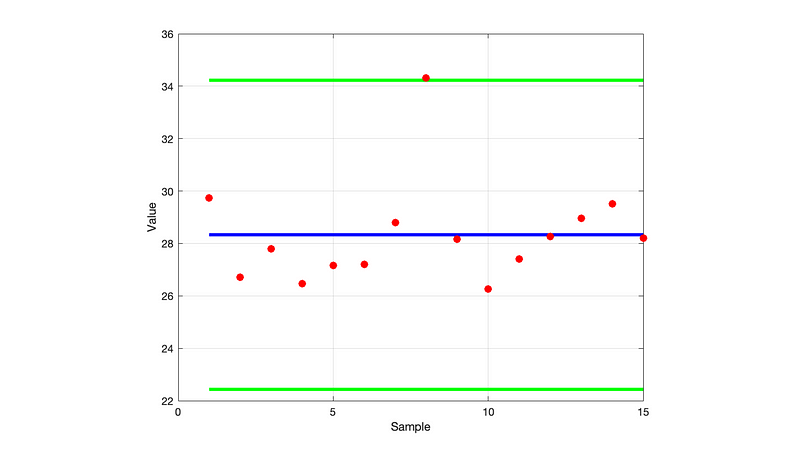
By drawing the boundary lines using the example above, you can see that one data point is actually an outlier:

The calculation is also easy to implement in Python:

lower_limit = 'dataset'.mean() - 3*'dataset'.std()
upper_limit = 'dataset'.mean() + 3*'dataset'.std()

Let’s look at the second example above, where the case was more difficult. Based on the calculation, the mean = 0, std = 97.5, thus the upper limit is 292.5 and the lower limit is -292.5, as you can see on the figure below.

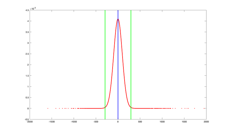
In this last example, it may appear that a significant amount of data points fall outside the boundaries, so we need to delete a large amount of data. Keep in mind, however, that statistically this is still only 0.28% of the total amount of data, and deleting it is usually not a problem.

c) Isolation Forest

Isolation forest is an algorithm to detect outliers. It works by constructing isolation trees to isolate outliers more efficiently than traditional methods. The algorithm leverages the concept that anomalies are easier to separate from the rest of the data due to their unique attribute values. This method is efficient for high-dimensional data and offers a scalable solution for detecting outliers in various domains.

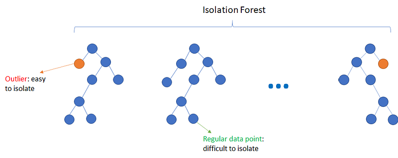
An important concept in this method is the isolation number. The isolation number is the number of splits needed to isolate a data point. The algorithm consists of the following iteration steps:

1. A point “a” to isolate is selected randomly.
2. A random data point “b” is selected that is between the minimum and maximum value and different from “a”.
3. If the value of “b” is lower than the value of “a”, the value of “b” becomes the new lower limit.
4. If the value of “b” is greater than the value of “a”, the value of “b” becomes the new upper limit.
5. This procedure is repeated as long as there are data points other than “a” between the upper and the lower limit.

It requires fewer splits to isolate an outlier than it does to isolate a non-outlier, i.e. an outlier has a lower isolation number in comparison to a non-outlier point. A data point is therefore defined as an outlier if its isolation number is lower than the threshold. The threshold is defined based on the estimated percentage of outliers in the data, which is the starting point of this outlier detection algorithm. This means that the normal distribution limits defined above can be a good starting point here.

In Python, you can easily implement the Isolation Forest algorithm with the SciKit-learn library:

from sklearn.ensemble import IsolationForest
clf = IsolationForest(random_state=101).fit('dataset')
clf.predict('dataset')

2) Identify Multivariate Outliers

Let’s move on to the identification of multivariate outliers. Here we need to examine the data series along several axes, so other methods are needed.

Let’s quickly look at why this is important.

Let us say we are understanding the relationship between height and weight. So, we have univariate and multivariate distributions too. According to the box plot and the IQR method, we do not have any outlier. Now look at the scatter plot. Here, we have two values below and one above the average in a specific segment of weight and height.

Therefore, we can see that the above methods cannot be used for multivariate variables. Instead of those, we can effectively use the DBSCAN algorithm.

a) DBSCAN

DBSCAN (Density-Based Spatial Clustering of Applications with Noise), captures the insight that clusters are dense groups of points. The idea is that if a particular point belongs to a cluster, it should be near to lots of other points in that cluster. Based on this consideration, the algorithm is well suited for outlier detection, as these points are located far from the other data point clusters.

To understand the algorithm, firstly we have to define p core point and the min_samples as a hyperparameter. This is simply the minimum number of core points, p needed in order to form a cluster. The second important hyperparameter is eps. This is the maximum distance between two samples for them to be considered as in the same cluster.

Now if p is a core point, then it forms a cluster together with all points (core or non-core) that are reachable from it in the eps range. Each cluster contains at least one core point, non-core points can be part of a cluster, but they form its ‘edge’, since they cannot be used to reach more points. Here again, you can use the normal distribution as a good starting point for setting the hyperparameters.

The example shows how dense data points form separate groups. At the same time, data points that are spaced away from each other do not belong to any of the groups, they will be the outlier values.

You can find here more interesting visualizations of how the clusters are generated:

You can use SciKit-learn library here too:

from sklearn.cluster import DBSCAN
clustering = DBSCAN(eps=3, min_samples=2).fit('dataset')
clustering.labels_ #label '-1' contains the outlier values

Conclusion

And that’s it. There are also more advanced methods for the above mentioned methods, but in most cases the simple algorithms presented here are sufficient to detect outlier values properly.

I hope that the above summary has been helpful for you.

If you found this article interesting, your support by following steps will help me spread the knowledge to others:

👏 Give me a clap

👀 Follow me

🗞️ Read articles on Medium

#learning #outliers #dataanalysis #datascience #python