Free AI web copilot to create summaries, insights and extended knowledge, download it at here

6469

Abstract

market dynamics. This is where feature engineering becomes invaluable. By transforming and synthesizing the raw data using established technical indicators, we can provide the model with enriched insights that could explain underlying market patterns and trends. Such enriched data can significantly improve the model’s ability to anticipate future price movements.</p><p id="07ea">For this forecast, we will utilize a couple of technical indicators for our feature engineering like RSI, MACD, Bollinger Bands, Parabolic SAR, and Stochastic Oscillator. Additionally, we introduce lag features to capture temporal dependencies, ensuring our model benefits from both current and historical contexts.</p><p id="f61d"><b>Let’s calculate the features we will utilize in this forecast</b></p><div id="d4ed"><pre><span class="hljs-comment"># Compute RSI</span> df[<span class="hljs-string">'momentum_rsi'</span>] = RSIIndicator(close=df[<span class="hljs-string">'Close'</span>]).rsi()

<span class="hljs-comment"># Compute MACD</span> macd = MACD(close=df[<span class="hljs-string">'Close'</span>]) df[<span class="hljs-string">'trend_macd'</span>] = macd.macd() df[<span class="hljs-string">'trend_macd_signal'</span>] = macd.macd_signal() df[<span class="hljs-string">'trend_macd_diff'</span>] = macd.macd_diff()

<span class="hljs-comment"># Compute Bollinger Bands</span> bollinger = BollingerBands(close=df[<span class="hljs-string">'Close'</span>]) df[<span class="hljs-string">'volatility_bbm'</span>] = bollinger.bollinger_mavg() df[<span class="hljs-string">'volatility_bbl'</span>] = bollinger.bollinger_lband() df[<span class="hljs-string">'volatility_bbh'</span>] = bollinger.bollinger_hband()

<span class="hljs-comment"># Compute Parabolic SAR</span> psar = PSARIndicator(high=df[<span class="hljs-string">'High'</span>], low=df[<span class="hljs-string">'Low'</span>], close=df[<span class="hljs-string">'Close'</span>]) <span class="hljs-comment"># Assuming you have 'High' and 'Low' columns in your df</span> df[<span class="hljs-string">'trend_psar'</span>] = psar.psar()

<span class="hljs-comment"># Compute Stochastic Oscillator</span> stochastic = StochasticOscillator(high=df[<span class="hljs-string">'High'</span>], low=df[<span class="hljs-string">'Low'</span>], close=df[<span class="hljs-string">'Close'</span>]) <span class="hljs-comment"># Assuming you have 'High' and 'Low' columns</span> df[<span class="hljs-string">'momentum_stoch'</span>] = stochastic.stoch() df[<span class="hljs-string">'momentum_stoch_signal'</span>] = stochastic.stoch_signal()

<span class="hljs-comment"># Create Lag Features</span> df[<span class="hljs-string">'Close_Lag1'</span>] = df[<span class="hljs-string">'Close'</span>].shift(<span class="hljs-number">1</span>)

<span class="hljs-comment"># Drop NaN values introduced due to lag features and indicators</span> df = df.dropna()

<span class="hljs-comment"># Define features and target</span> X = df[[<span class="hljs-string">'momentum_rsi'</span>, <span class="hljs-string">'trend_macd'</span>, <span class="hljs-string">'trend_macd_signal'</span>, <span class="hljs-string">'trend_macd_diff'</span>, <span class="hljs-string">'volatility_bbm'</span>, <span class="hljs-string">'volatility_bbl'</span>, <span class="hljs-string">'volatility_bbh'</span>, <span class="hljs-string">'trend_psar'</span>, <span class="hljs-string">'momentum_stoch'</span>, <span class="hljs-string">'momentum_stoch_signal'</span>, <span class="hljs-string">'Close_Lag1'</span>]] y = df[<span class="hljs-string">'Close'</span>]</pre></div><p id="712f">The above code is organizing the dataset <code>df</code> into input features and a target variable for our model. The input features, captured under <code>X</code>, consist of various the features we calculated on and previously defined. The target variable, denoted by <code>y</code>, is the <code>Close</code> column, representing the daily closing price of EUR/USD, which our model aims to predict based on the provided features.</p><p id="bdfb"><b>Model Initialization and Training</b></p><div id="a7d2"><pre><span class="hljs-comment"># Initialize the model</span> model = xgb.XGBRegressor( learning_rate=<span class="hljs-number">0.75</span>, n_estimators=<span class="hljs-number">200</span>, max_depth=<span class="hljs-number">5</span>, subsample=<span class="hljs-number">0.9</span>, colsample_bytree=<span class="hljs-number">0.8</span>, colsample_bylevel=<span class="hljs-number">0.8</span>, gamma=<span class="hljs-number">0</span>, min_child_weight=<span class="hljs-number">1</span> )

<span class="hljs-comment"># Train the model</span> model.fit(X_train, y_train)</pre></div><p id="7ce9">Continuing from the previously discussed data preparation, this section of code dives into the model initialization and training phases using XGBoost. The <code>xgb.XGBRegressor()</code> initializes a regression model with specified hyperparameters to optimize the forecast. Key parameters include a learning rate of <code>0.75</code>, which determines the step size at each iteration while optimizing, <code>200</code> estimators or trees, and a maximum depth of <code>5</code> for each tree, among others. These hyperparameters play a role in controlling the model’s complexity and fit to the data.</p><p id="4e91">After initializing, the model is trained on the <code>X_train</code> and <code>y_train</code> datasets using the <code>fit</code> method. This step allows the model to learn the underlying patterns from the training data, preparing it to make future predictions on unseen data.</p><p id="95cf"><b>Performance Evaluation and Testing</b></p><div id="a823"><pre><span class="hljs-comment"># Predict on the test set</span> y_pred = model.predict(X_test)

<span class="hljs-comment"># Calculate performance metrics</span> mae = mean_absolute_error(y_test, y_pred) mse = mean_squared_error(y_test, y_pred) rmse = np.sqrt(mse)

<span class="hljs-built_in">print</span>(<span class="hljs-string">f"Mean Absolute Error: <span class="hljs-subst">{mae}</span>"</span>) <span class="hljs-built_in">print</span>(<span class="hljs-string">f"Mean Squared Error: <span class="hljs-subst">{mse}</span>"</span>) <span class="hljs-built_in">print</span>(<span class="hljs-string">f"Root Mean Squared Error: <span class="hljs-subst">{rmse}</span>"</span>)

y_train_pred = model.predict(X_train)</pre></div><p id="8c56">After training the

Options

model on the historical data we evaluate its performance on unseen or test data. Using the <code>predict</code> method of the trained model, predictions (<code>y_pred</code>) are generated for the test dataset <code>X_test</code>. Subsequently, to assess the accuracy and reliability of these predictions, various performance metrics are computed:</p><ul><li><b>The Mean Absolute Error (MAE)</b> provides an average magnitude of errors between predicted and actual values.</li><li><b>The Mean Squared Error (MSE) </b>squares these errors to emphasize larger discrepancies.</li><li><b>Root Mean Squared Error (RMSE) </b>is the square root of MSE, providing error in the same units as the original data.</li></ul><p id="c92b">These metrics are then printed for clear visibility. We concludes by also predicting on the training set (<code>X_train</code>) with <code>y_train_pred</code>, to further analyze and compare the model’s performance on both training and test datasets.</p><p id="44c0">The following output displays the performance metricswhich assess the accuracy of our model’s predictions:</p><div id="6743"><pre><span class="hljs-attribute">Mean</span> Absolute Error: <span class="hljs-number">0</span>.<span class="hljs-number">009141215039947168</span> <span class="hljs-attribute">Mean</span> Squared Error: <span class="hljs-number">0</span>.<span class="hljs-number">000303615460154008</span> <span class="hljs-attribute">Root</span> Mean Squared Error: <span class="hljs-number">0</span>.<span class="hljs-number">017424564848340058</span></pre></div><ul><li><b>Mean Absolute Error (MAE): </b>At 0.0091, it shows the model’s average absolute deviation from the actual values.</li><li><b>Mean Squared Error (MSE):</b> With a value of 0.0003036, it indicates the average squared error, emphasizing larger mistakes.</li><li><b>Root Mean Squared Error (RMSE):</b> At 0.0174, it provides the average error in the original unit, illustrating the typical magnitude of error.</li></ul><p id="7500">The relatively low values across these metrics suggest that the model has a good degree of accuracy in its predictions. The model appears to be reliably forecasting the target variable, depicted with minimal deviations in the forecasted data when compared to the actual data.</p><p id="be3b"><b>Data Visualization</b></p><div id="2b49"><pre><span class="hljs-comment"># Create a new DataFrame for visualization</span> viz_df = pd.DataFrame({<span class="hljs-string">'True'</span>: y_test, <span class="hljs-string">'Predicted'</span>: y_pred})

<span class="hljs-comment"># Concatenate the training data for a complete view</span> viz_df_train = pd.DataFrame({<span class="hljs-string">'True'</span>: y_train, <span class="hljs-string">'Predicted'</span>: y_train_pred}) viz_df = pd.concat([viz_df_train, viz_df])

<span class="hljs-comment"># Plot the results</span> plt.figure(figsize=(<span class="hljs-number">14</span>, <span class="hljs-number">7</span>)) plt.plot(viz_df[<span class="hljs-string">'True'</span>], label=<span class="hljs-string">'True'</span>, color=<span class="hljs-string">'blue'</span>) plt.plot(viz_df[<span class="hljs-string">'Predicted'</span>], label=<span class="hljs-string">'Predicted'</span>, color=<span class="hljs-string">'red'</span>, alpha=<span class="hljs-number">0.7</span>) plt.title(<span class="hljs-string">'EUR/USD Forecast: True vs Predicted'</span>) plt.legend() plt.grid(<span class="hljs-literal">True</span>) plt.show()</pre></div><figure id="ce5c"><img src="https://cdn-images-1.readmedium.com/v2/resize:fit:800/1*cLlTTCFRMZqUBQIUBeya0g.png"><figcaption></figcaption></figure><p id="62e5">The visual representation of the EUR/USD currency pair’s forecasted versus actual values offers an insightful glimpse into the model’s capabilities. The close alignment between the blue <code>True</code> line and the red <code>Predicted</code> line for most of the chart affirms the model’s strong predictive proficiency, especially given the low Mean Absolute Error (MAE) of 0.0091. The few areas where deviations occur resonate with the Root Mean Squared Error (RMSE) of 0.0174, indicating the average magnitude of error.</p><p id="ba85">Notably, the small segment towards the right end, where predictions seem to diverge slightly, underscores the challenges of exact currency forecasting. Nevertheless, the model, as depicted in the graph and corroborated by the performance metrics, has shown remarkable accuracy in capturing the nuances of the EUR/USD exchange rate’s movements.</p><h1 id="fe27">Conclusion</h1><p id="3036">In conclusion, this exploration into Forex forecasting has underscored the critical interplay between data preprocessing, feature engineering, and model selection. Through this model we found that XGBoost in predicting the EUR/USD currency pair stands out, demonstrating the algorithm’s robustness and adaptability. Finally, the precision showcased by our model reinforces XGBoost’s reputation as an efficient tool to forecast financial data.</p><p id="0141">Read more of my stories here:</p><div id="c60c" class="link-block"> <a href="https://algocraft.xyz/eur-usd-forecasting-simplified-an-lstm-users-guide-337ccdda6158"> <div> <div> <h2>EUR/USD Forecasting Simplified: an LSTM User’s Guide</h2> <div><h3>LSTM, or Long Short-Term Memory, is a specialized type of Recurrent Neural Network (RNN) designed to recognize patterns…</h3></div> <div><p>algocraft.xyz</p></div> </div> <div> <div style="background-image: url(https://miro.readmedium.com/v2/resize:fit:320/1*EUIE-cUkt3x2AqBX5nUotA.jpeg)"></div> </div> </div> </a> </div><div id="a6a6" class="link-block"> <a href="https://algocraft.xyz/how-to-get-131-return-with-mean-reversion-trading-strategy-from-stock-selection-to-backtesting-c623870adf31"> <div> <div> <h2>How to Get a 131% Return with Mean Reversion Trading Strategy: From Stock Selection to Backtesting</h2> <div><h3>undefined</h3></div> <div><p>undefined</p></div> </div> <div> <div style="background-image: url(https://miro.readmedium.com/v2/resize:fit:320/0*o95y-D4ETf1Geqx3)"></div> </div> </div> </a> </div></article></body>

A Place to Live and Die

Lucas Winslow, the tree whisperer

When Lucas first saw the cabin he could immediately feel the sublime vibrations. After almost a year of searching for the perfect place in which to spend the rest of his life he had come to rely on his inner senses and what their immediate responses were. So many times a real estate agent had led him to a home that had very weak or dead vibrations. Feeling that, Lucas usually cut the tour short.

When he sensed life-affirming vibrations he would proceed to extensively tour the home and property. Once beyond initial vibratory reads from his inner senses then there were countless other considerations to be validated, both from his inner senses, outer senses and the desires in his mind and heart.

Lucas was very, very picky. After all, he was looking for a place to both live and die. He wanted everything to be perfect.

Sitting in the passenger seat of the real estate agent’s car as they drove through the undulating pinon/juniper woodland, Lucas could feel excitement welling up inside him. In previous meditations, he had attempted to project himself into the future to get glimpses of his final home and in those vague projections he could tell that the land to the north of that imagined home was covered by the very biome he was now traveling through. He lowered the car window so that he could smell the land.

The elevation seemed right, too; not too high, where the growing season is too short, and not too low where the summer heat would be too stifling. They were driving through the lower reaches of the pinon/juniper woodland, well below the tall forests of the mountains to the north yet still above the desert lowlands to the south.

The real estate agent pulled into a small dirt and gravel parking area and parked her car. Turning to Lucas, she said, “I think you’re gonna like this place.” (She had said that many times before.)

Getting out of the car, Lucas walked to the front of the car where he met up with the real estate agent. His eyes were scanning the property in all directions.

“You can’t see the cabin from here. It’s on the side of the hill beyond those trees,” she pointed. “I think the only downside is that the parking isn’t right up next to the house. You’ve actually gotta walk a little ways.”

“Oh, I kind of like that.”

“Well, follow me. This path leads down to the house. Because the house is a little lower than the road you won’t have to be bothered much by traffic noise — not that there’s much traffic on that out-of-the-way road. I know you said you were looking for a quiet place. Well, this place is super quiet.”

A lone black and white magpie perched atop a pinon pine watched Lucas and the real estate woman walk the dirt path down to the cabin. The real estate agent was oblivious of the bird but Lucas could not help but notice it and sent it some love.

“The cabin is small, like you wanted, and it has plenty of windows, like you wanted, but it has all the amenities and is in very good condition. Actually, I don’t think we can technically call it a cabin since it’s made of adobe, not wood. Plus, it’s sort of built into the side of the hill.”

As the dwelling came into view Lucas stopped in his tracks. The hairs on his arms were standing upright.

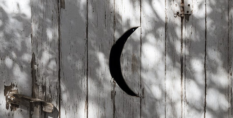
“Now in addition to the house there is that tool shed down by the orchard and there is also that wooden outhouse over there. But don’t worry, the house has a well and indoor plumbing so you won’t have to use the outhouse. The house was originally built almost a hundred years ago and back then it had no plumbing but the last owner put in plumbing but kept the outhouse I guess for aesthetic reasons or something. I guess it’s kind of cute, especially with that crescent moon carved into the door.”

“Oh, I really like outhouses.”

The agent screwed up her face, “Really?”

“Yes, it’s been a few decades since I’ve used one but I have fond memories. So is that orchard down there in the valley part of the property?”

“Oh yes. The property includes twenty-two acres. It begins at the road and goes down into the little valley all the way to a small creek that you can’t see because of the orchard. It includes the entire orchard as well as that fenced pasture over there and that field between the orchard and the pasture. It just looks like a field of weeds right now because no crops have been grown there in a few years.”

“Excellent.”

“There is also that ditch, or acequia, that runs through the property between the house and the orchard and fields below. I think it’s dry now but it has water at certain times of the year and that is used to irrigate the orchard and fields below. Plus, of course, as I said, the property also has a well. Okay, here we are at the house.”

There was a large flagstone patio in front of the house and as they stood on it Lucas took a quick reading with his inner compass. The house faced southward overlooking the little valley and orchard below. Looking back and forth between east and west, Lucas could see that there were no obstructions to the view of both horizons. This was crucially important to Lucas in regard to his sunrise and sunset rituals.

Lucas and the real estate agent then went inside the house. Almost the entire south side of the building was covered with large and tall windows. There were also plenty of windows on both the east and west sides of the house. Being partially built into the hillside, there were no windows facing north.

The home was very open with very few walls. There was a small upper level sleeping area that was open to the rest of the house. Underneath this sleeping area were the only walled off rooms; a bathroom and a very large closet. An open kitchen was on the east side of the cabin and a sitting area with fireplace was on the west side.

Lucas looked at the area in front of the south side windows and visualized his writing desk there. He would be able to sit at his desk and look out over a beautiful rural panorama. Plus, he would be situated to the north of his laptop. It was perfect.

Lucas took a deep breath. The place had a very pleasant earthy scent of wood and adobe. The vibes were very soothing.

“So do you like it?”

“I love it!” Lucas spun around taking in everything inside the little cabin/home. “Seriously, this is feeling really, really good. I feel so at home here.”

The real estate agent smiled.

“There is one thing I’ve got to do first, though, before I make a decision.”

“Okay.”

“I’ve got to go down into the orchard and talk to the trees.”

Would Lucas buy the property? Would he spend the rest of his life there? And what would the trees tell him?

And what would he tell the trees?

More Lucas Winslow stories:

The Silent Teacher

Who may or may not still be alive

medium.com

The First Time Steve Showed Up

And Lucas thought he would be all alone

medium.com