Recommendation System

A Performant Recommender System Without Cold Start Problem

When collaboration and content-based recommenders merge

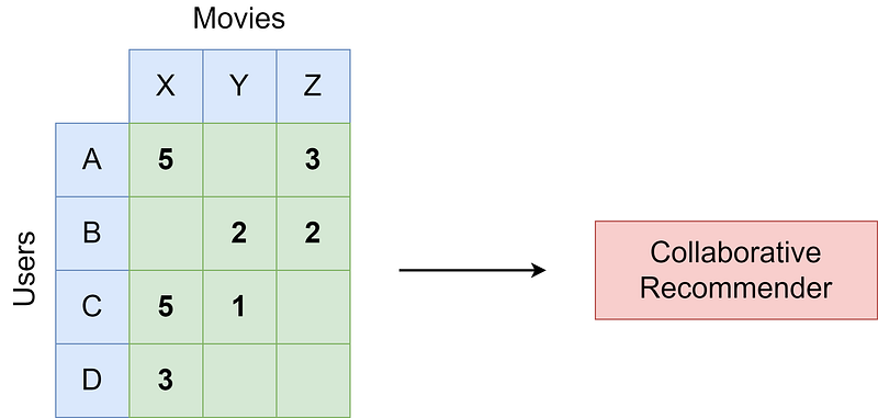
Perhaps the most famous recommender system is the so-called matrix factorization. In this collaborative recommender, users and items are represented with an embedding, which is nothing more but a vector of numbers. The intuition is that the dot product of the user and the item embedding should result in the rating that the user would give this item.

If you are not yet familiar with these concepts, I recommend (😉) reading my other article before you proceed since I explain many concepts and code snippets there.

The Cold Start Problem

Purely collaborative recommender systems such as matrix factorization have the advantage that you can usually immediately build them even without having too much data about your users and movies/articles/items you want to recommend. You only have to know who rated what and how; for example, user B gave movie Y a rating of 2 stars.

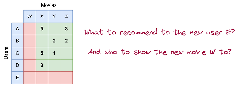
However, they fall short when you have new users or items that you want to make predictions for since the model had no possibility of learning anything for them, leaving you with basically random recommendations for them — the dreaded cold start problem. Let us assume that another user E registers, and we also add a new movie W to the database.

In this article, I will show you a simple way to mitigate the cold start problem by incorporating more features about the users and items — this is the content-based component we will bake into our model. Using actual content data, such as user age or a movie genre, produces models that can deal with new users or movies in a better way.

Back to MovieLens

As in my last article, I will use the MovieLens dataset that provides us with user-movie ratings. Furthermore, it even contains some more user and movie features, and while we ignored these in the last article, we will use them today to build an even better model!

You can find the code on my Github.

Following the last article let us

1. grab the data using tensorflow-datasets
2. make a dataframe out of it and change some column types, and
3. sort it according to the time to conduct a temporal train-test split

import tensorflow_datasets as tfds


data = tfds.load("movielens/1m-ratings")
df = tfds.as_dataframe(data["train"])

filtered_data = (
    df
    .sort_values("timestamp") # for a temporal train-eval-test split
    .astype(
        {
            "bucketized_user_age": int,
            "movie_id": int,
            "movie_title": str,
            "user_gender": int,
            "user_id": int,
            "user_occupation_label": int,
            "user_occupation_text": str,
            "user_rating": int,
            "user_zip_code": str,
        }
    )
    .drop(columns=["timestamp"])
)

# temporal train-eval-test split
train = filtered_data.iloc[:80000]
evaluation = filtered_data.iloc[80000:90000]
test = filtered_data.iloc[90000:]

X_train = train.drop(columns=["user_rating"])
y_train = train["user_rating"]
X_eval = evaluation.drop(columns=["user_rating"])
y_eval = evaluation["user_rating"]
X_test = test.drop(columns=["user_rating"])
y_test = test["user_rating"]

The filtered_data dataframe

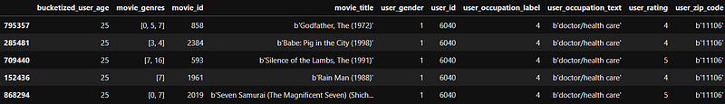
tells us that besides user_id, movie_id and the target user_rating we have the user features

• bucketized_user_age
• user_gender
• user_occupation_label
• user_occupation_text
• user_zip_code

and the movie features

• movie_genres
• movie_title

Using some stereotypes:

Intuitively, these features should help a lot since a model could learn things like “Women like dramas” or “Young people dislike old movies”.

We will now find out how to use all of these additional features via a simple network architecture called LightFM. The name was chosen by Maciej Kula in his well-written paper Metadata Embeddings for User and Item Cold-start Recommendations [1]. Please give it a read!

LightFM is a hybrid of a collaborative as well as a content-based recommender since it uses ratings as well as user and item features.

The Simple Idea of LightFM

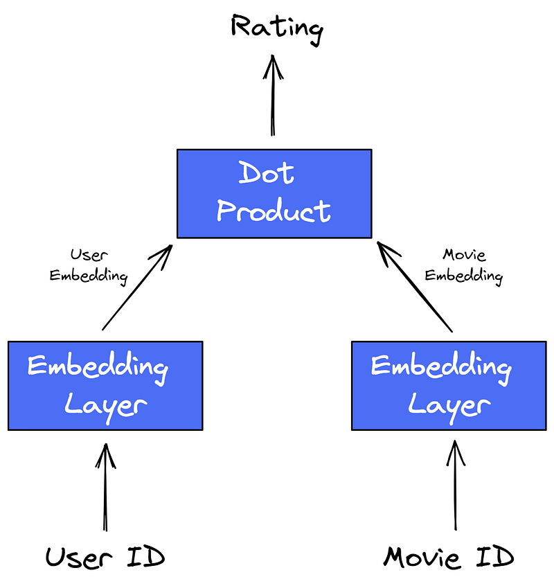
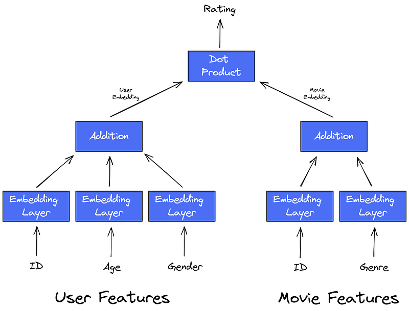
Let us first recap what our simple matrix factorization looked like, omitting biases. In our old recommender, we used the user_id and movie_id, embedded both, and computed the dot product to calculate the rating.

For LightFM, it works like this:

1. We embed all the features that we have, user and movie features.
2. The user (movie) embedding is the sum of all these user (movie) feature embeddings.

That’s it already! For some subset of features, the network architecture could look like this:

Advantages

The good thing about this approach is that even if you get a new user or movie into the database, you can create meaningful embeddings as long as you know their features (contents). You will not know the embeddings for the IDs — the main problem in the matrix factorization approach — but we hope that the other embeddings make up for it. In a cold start setting, user_id or movie_id are unknown, but we can still give them some default embedding.

Implementation in TensorFlow

With only the two IDs as input, it is sufficient to explicitly type out an input, encoding, embedding, and bias. However, for our number of features, it makes sense to define some config first and then use loops.

Note: We will omit movie_title and movie_genres since we have to treat them differently than the rest. However, I will tell you things you can do to incorporate these features as well.

features_config = {
    "user_id": {"entity": "user", "dtype": tf.int64},
    "bucketized_user_age": {"entity": "user", "dtype": tf.int64},
    "user_gender": {"entity": "user", "dtype": tf.int64},
    "user_occupation_label": {"entity": "user", "dtype": tf.int64},
    "movie_id": {"entity": "movie", "dtype": tf.int64},
    "user_zip_code": {"entity": "user", "dtype": tf.string},
    "user_occupation_text": {"entity": "user", "dtype": tf.string},
}

for name, config in features_config.items():
    if config["dtype"] == tf.int64:
        config["encoding_layer_class"] = tf.keras.layers.IntegerLookup
    elif config["dtype"] == tf.string:
        config["encoding_layer_class"] = tf.keras.layers.StringLookup
    else:
        raise Exception

    config["vocab"] = train[name].unique()

We now have an extensive configuration dictionary that tells us about each feature

• which input dtype the input layer needs,
• if the features belong to the movie or user features,
• which lookup layer is needed, i.e. IntegerLookup for integer features and StringLookup for string features,
• and the vocabulary, i.e., the unique classes per feature.

Then, we can define a TensorFlow model that does what we have seen in the LightFM architecture image:

# define input layers for each feature
inputs = {
    name: tf.keras.layers.Input(shape=(1,), name=name, dtype=config["dtype"])
    for name, config in features_config.items()
}

# encode all features as integers via the lookup layers
inputs_encoded = {
    name: config["encoding_layer_class"](vocabulary=config["vocab"])(inputs[name])
    for name, config in features_config.items()
}

# create embeddings for all features
embeddings = {
    name: tf.keras.layers.Embedding(
        input_dim=len(config["vocab"]) + 1,
        output_dim=32,
    )(inputs_encoded[name])
    for name, config in features_config.items()
}

# create embeddings for all features
biases = {
    name: tf.keras.layers.Embedding(input_dim=len(config["vocab"]) + 1, output_dim=1)(
        inputs_encoded[name]
    )
    for name, config in features_config.items()
}

# compute the user embedding as the sum of all user feature embeddings
user_embedding = tf.keras.layers.Add()(
    [
        embeddings[name]
        for name, config in features_config.items()
        if config["entity"] == "user"
    ]
)

# compute the movie embedding as the sum of all movie feature embeddings
movie_embedding = tf.keras.layers.Add()(
    [
        embeddings[name]
        for name, config in features_config.items()
        if config["entity"] == "movie"
    ]
)

# compute the user bias as the sum of all user feature biases
user_bias = tf.keras.layers.Add()(
    [
        biases[name]
        for name, config in features_config.items()
        if config["entity"] == "user"
    ]
)

# compute the movie bias as the sum of all movie feature biases
movie_bias = tf.keras.layers.Add()(
    [
        biases[name]
        for name, config in features_config.items()
        if config["entity"] == "movie"
    ]
)

# do the exact same thing as in matrix factorization, 
# i.e. compute the dot product of the user and movie embedding,
# add the user and movie bias, and squash the result into the range [1, 5]
dot = tf.keras.layers.Dot(axes=2)([user_embedding, movie_embedding])
add = tf.keras.layers.Add()([dot, user_bias, movie_bias])
flatten = tf.keras.layers.Flatten()(add)
squash = tf.keras.layers.Lambda(lambda x: 4 * tf.nn.sigmoid(x) + 1)(flatten)

model = tf.keras.Model(
    inputs=[inputs[name] for name in features_config.keys()], outputs=squash
)

model.compile(loss="mse", metrics=[tf.keras.metrics.MeanAbsoluteError()])

I know this is quite hefty. But there should be no big surprises if you also read my other article about embedding-based recommenders. We are ready to train the model!

model.fit(
    x={name: X_train[name].values for name in features_config.keys()},
    y=y_train.values,
    batch_size=256,
    epochs=100,
    validation_data=(
        {name: X_eval[name].values for name in features_config.keys()},
        y_eval.values,
    ),
    callbacks=[tf.keras.callbacks.EarlyStopping(patience=1, restore_best_weights=True)],
)

# Output:
# [...]
# Epoch 6/100
# 313/313 [==============================] - 1s 3ms/step - loss: 0.7626 - mean_absolute_error: 0.6836 - val_loss: 0.9836 - val_mean_absolute_error: 0.7985

The performance on the test set:

model.evaluate(
    x={name: X_test[name].values for name in features_config.keys()},
    y=y_test.values,
    batch_size=1_000_000,
)

# Output:
# 1/1 [==============================] - 1s 667ms/step - loss: 1.0153 - mean_absolute_error: 0.8135

You can also try out the matrix factorization in this setting; you only have to change the features_config dictionary to

features_config = {
    "user_id": {"entity": "user", "dtype": tf.int64},
    "movie_id": {"entity": "movie", "dtype": tf.int64},
}

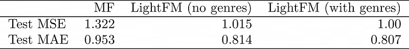
by deleting some rows and then executing the rest of the code. The results, in this case, are a test MSE of 1.322 and an MAE of 0.953, which is much worse than the LightFM results. This looks great!

Dealing With The Movie Genre

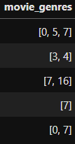
So far, we have ignored the perhaps extremely informative column movie_genres because it is a bit harder to handle than the categorical variables since here we have a list of integers instead of just one integer. So, we have to make up some logic to deal with this.

The easiest thing to do with this is to make an embedding for each genre and then take the mean of them. You can use the GlobalAveragePooling1D layer for this.

In order to realize this idea in code, do the following:

# new movie embeddings
all_movie_genres = train["movie_genres"].explode().unique().astype(int) # get all different genres
movie_genres_input = tf.keras.layers.Input(shape=(None,), name="movie_genres")
movie_genres_as_integer = tf.keras.layers.IntegerLookup(vocabulary=all_movie_genres)(movie_genres_input)
movie_genres_embeddings = tf.keras.layers.Embedding(input_dim=len(all_movie_genres) + 1, output_dim=32)(movie_genres_as_integer)
movie_genres_biases = tf.keras.layers.Embedding(input_dim=len(all_movie_genres) + 1, output_dim=1)(movie_genres_as_integer)
movie_genres_embedding = tf.keras.layers.GlobalAveragePooling1D(keepdims=True)(movie_genres_embeddings)
movie_genres_bias = tf.keras.layers.GlobalAveragePooling1D(keepdims=True)(movie_genres_biases)

movie_embedding = tf.keras.layers.Add()(
    [
        embeddings[name]
        for name, config in features_config.items()
        if config["entity"] == "movie"
    ] + [movie_genres_embedding] # add the movie genres embedding here as well
)

# new movie bias
movie_bias = tf.keras.layers.Add()(
    [
        biases[name]
        for name, config in features_config.items()
        if config["entity"] == "movie"
    ] + [movie_genres_bias] # add the movie genres bias here as well
)

# add the movie inut to the inputs
model = tf.keras.Model(
    inputs=[inputs[name] for name in features_config.keys()] + [movie_genres_input], outputs=squash
)

The rest stays the same. You only have to add the feature movie_genres to the model during fit, evaluation, and testing as well. The shape of the genres is a bit difficult since the lists don’t have the same length, so TensorFlow has trouble turning this into a regular tensor. Luckily, TensorFlow still got us covered by providing ragged tensors via tf.ragged.constant that can handle these variable-size tensors.

model.fit(
    x={
        **{name: X_train[name].values for name in features_config.keys()},
        "movie_genres": tf.ragged.constant(X_train["movie_genres"].values)
    },

# [...]

Fitting and evaluating the model on the test set shows yet another improvement, although smaller than expected. The MSE is about 1.0, and MAE is about 0.807.

Dealing with the Movie Title

Another interesting feature we have ignored so far since it contains information about the movie franchise. With this information, we could make it easy for the model to learn that some users like all the Batman movies a lot, for example. Coding this is homework for you, though. One way to do this is to split the title strings into a list of words and then proceed as we did with the genres. You can even use sentence encoders, transformer-like architecture, LSTMs, or anything else to turn a text into an embedding.

Making Predictions

You can make a prediction by providing all the necessary features like this:

query = {
    "user_id": tf.constant([-1]), # unknown user!
    "bucketized_user_age": tf.constant([18]),
    "user_gender": tf.constant([0]),
    "user_occupation_label": tf.constant([12]),
    "movie_id": tf.constant([1]),
    "user_zip_code": tf.constant(["b'65712'"]),
    "user_occupation_text": tf.constant(["b'writer'"]),
    "movie_genres": tf.ragged.constant([[1, 2, 3]])
}

model.predict(query)

# Output:
# array([[4.0875683]], dtype=float32)

Here, you can see that some unknown user who is young, has gender 0, occupation label 12, living in the 65712 zip code area, and is a writer would probably like the movie with id 1 that belongs to the genres 1, 2, and 3.

More Interesting Insights From The Paper

My small experiment showed that LightFM could increase the model performance, as also stated in [1]. This is great, although something you might have expected already since LightFM is a generalized version of matrix factorization.

In this regard, the paper author writes the following:

1. “In both cold-start and low-density scenarios, LightFM performs at least as well as pure content-based models, substantially outperforming them when either (1) collaborative information is available in the training set or (2) user features are included in the model.”
2. “When collaborative data is abundant (warm-start, dense user-item matrix), LightFM performs at least as well as the MF model.”
3. “Embeddings produced by LightFM encode important semantic information about features and can be used for related recommendation tasks such as tag recommendations.”

There is no proof of these statements, but he reached this conclusion by testing it on two datasets. Both datasets have binary labels, though, meaning that either the item was useful for the user or not. With binary labels, he chose the AUC as his evaluation metric and summarized his findings in this table:

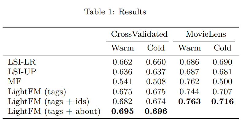
Here, we can also see that LightFM outperforms the other methods in the cold start and even the warm start setting. It is good to see that LightFM is not worse than MF in the warm start setting, but the main selling point is that LightFM completely destroys MF in the cold setting.

Remember: An AUC of 0.5 means random guessing in the sense that the probability that a randomly picked relevant item for some user scores higher than a randomly chosen non-relevant item for this user is 50%.

Conclusion

In this article, we have discussed how purely collaborative recommender systems, such as matrix factorization, have trouble when seeing new users or items, referred to as the cold start problem.

We can mitigate this problem once we have more information about users and items since the model can learn some general patterns, such as that young people dislike old movies. So, if we have a new user and know they are young, a good model should score older movies lower than newer ones.

Still, if this new user keeps rating movies, the model can adjust and learn to display old movies like Nosferatu if the user’s behavior indicates that this might be a good fit.

A model with these desirable properties feels a bit Bayesian to me:

The user and item feature embeddings serve as a kind of prior that has a great influence on the predictions as long as we don’t have interaction data. As interactions come in, this prior gets changed.

However, it is an interesting question whether the user and item features lose their relevance once we have a dense rating matrix, e.g., if each user rated 95% of all movies.

Anyway, LightFM is a good candidate for such a model, as indicated by my and the paper author’s experiments. LightFM beats MF, especially in the cold start setting on our selected datasets. If the cold start is not an issue, the improvements are minor and might even be just statistical noise.

You can also try the paper author’s implementation of LightFM.

References

[1] M. Kula, Metadata Embeddings for User and Item Cold-start Recommendations (2015), arXiv preprint arXiv:1507.08439

I hope that you learned something new, interesting, and useful today. Thanks for reading!

If you have any questions, write me on LinkedIn!

And if you want to dive deeper into the world of algorithms, give my new publication All About Algorithms a try! I’m still searching for writers!