A Minimal Working Example for Continuous Policy Gradients in TensorFlow 2.0

A simple example for training Gaussian actor networks. Defining a custom loss function and applying the GradientTape functionality, the actor network can be trained using only a few lines of code.

At the root of all the sophisticated actor-critic algorithms that are designed and applied these days is the vanilla policy gradient algorithm, which essentially is an actor-only algorithm. Nowadays, the actor that learns the decision-making policy is often represented by a neural network. In continuous control problems, this network outputs the relevant distribution parameters to sample appropriate actions.

With so many deep reinforcement learning algorithms in circulation, you’d expect it to be easy to find abundant plug-and-play TensorFlow implementations for a basic actor network in continuous control, but this is hardly the case. Various reasons may exist for this. First, TensorFlow 2.0 was released only in September 2019, differing quite substantially from its predecessor. Second, most implementations focus on discrete action spaces rather than continuous ones. Third, there are many different implementations in circulation, yet some are tailored such that they only work in specific problem settings. It can be a tad frustrating to plow through several hundred lines of code riddled with placeholders and class members, only to find out the approach is not suitable to your problem after all. This article — based on our ResearchGate note [1] — provides a minimal working example that functions in TensorFlow 2.0. We will show that the real magic happens in only three lines of code!

Some mathematical background

In this article, we present a simple and generic implementation for an actor network in the context of the vanilla policy gradient algorithm REINFORCE [2]. In the continuous variant, we usually draw actions from a Gaussian distribution; the goal is to learn an appropriate mean μ and a standard deviation σ. The actor network learns and outputs these parameters.

Let’s formalize this actor network a bit more. Here, the input is the state s or a feature array ϕ(s), followed by one or more hidden layers that transform the input, with the output being μ and σ. Once obtaining this output, an action a is randomly drawn from the corresponding Gaussian distribution. Thus, we have a=μ(s)+σ(s)ξ , where ξ ∼ 𝒩(0,1).

After taking our action a, we observe a corresponding reward signal v. Together with some learning rate α, we may update the weights into a direction that improves the expected reward of our policy. The corresponding update rule [2] — based on gradient ascent — is given by:

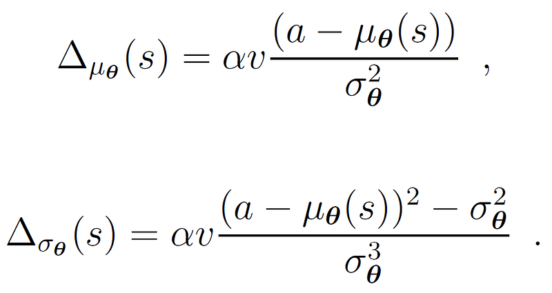
If we use a linear approximation scheme μ_θ(s)=θ^⊤ ϕ(s), we may directly apply these update rules on each feature weight. For neural networks, it may not be as straightforward how we should perform this update though.

Neural networks are trained by minimizing a loss function. We often compute the loss by computing the mean-squared error (squaring the difference between the predicted- and observed value). For instance, in a critic network the loss could be defined as (rₜ + Qₜ₊₁ - Qₜ)², with Qₜ being the predicted value and rₜ + Qₜ₊₁ the observed value. After computing the loss, we backpropagate it through the network, computing the partial losses and gradients required to update the network weights.

At first glance, the update equations have little in common with such a loss function. We simply try to improve our policy by moving into a certain direction, but do not have an explicit ‘target’ or ‘true value’ in mind. Indeed, we will need to define a ‘pseudo loss function’ that helps us update the network [3]. The link between the traditional update rules and this loss function become more clear when expressing the update rule into its generic form:

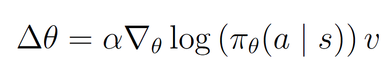
Transformation into a loss function is fairly straightforward. As the loss is only the input for the backpropagation procedure, we first drop the learning rate α and gradient ∇_θ. Furthermore, neural networks are updated using gradient descent instead of gradient ascent, so we must add a minus sign. These steps yield the following loss function:

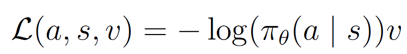
Quite similar to the update rule, right? To provide some intuition: remind that the log transformation yields a negative number for all values smaller than 1. If we have an action with a low probability and a high reward, we’d want to observe a large loss, i.e., a strong signal to update our policy into the direction of that high reward. The loss function does precisely that.

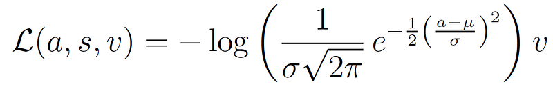
To apply the update for a Gaussian policy, we can simply substitute π_θ with the Gaussian probability density function (pdf) — note that in the continuous domain we work with pdf values rather than actual probabilities — to obtain the so-called weighted Gaussian log likelihood loss function:

TensorFlow 2.0 implementation

Enough mathematics for now, it’s time for the implementation.

We just defined the loss function, but unfortunately we cannot directly apply it in Tensorflow 2.0. When training a neural network, you may be used to something like model.compile(loss='mse',optimizer=opt), followed by model.fitormodel.train_on_batch, but this doesn’t work. First of all, the Gaussian log likelihood loss function is not a default one in TensorFlow 2.0 — it is in the Theano library for example[4] — meaning we have to create a custom loss function. More restrictive though: TensorFlow 2.0 requires a loss function to have exactly two arguments, y_true and y_predicted. As we just saw, we have three arguments due to multiplying with the reward. Let’s worry about that later though and first present our custom Guassian loss function:

So we have the correct loss function now, but we cannot apply it!? Of course we can — otherwise all of this would have been fairly pointless — it’s just slightly different than you might be used to.

This is where the GradientTapefunctionality comes in, which is a novel addition to TensorFlow 2.0 [5]. It essentially records your forward steps on a ‘tape’ such that it can apply automatic differentiation. The updating approach consists of three steps [6]. First, in our custom loss function we make a forward pass through the actor network — which is memorized — and calculate the loss. Second, with the function .trainable_variables, we recall the weights found during our forward pass. Subsequently, tape.gradient calculates all the gradients for you by simply plugging in the loss value and the trainable variables. Third, with optimizer.apply_gradients we update the network weights, where the optimizer is one of your choosing (e.g., SGD, Adam, RMSprop). In Python, the update steps look as follows:

So in the end, we only need a few lines of codes to perform the update!

Numerical example

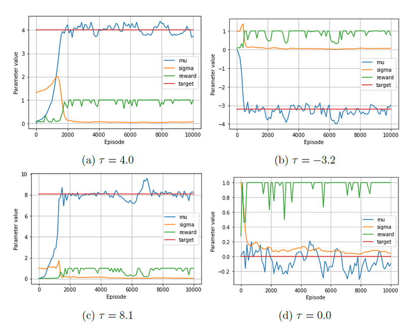
We present a minimal working example for a continuous control problem, the full code can be found on my GitHub. We consider an extremely simple problem, namely a one-shot game with only one state and a trivial optimal policy. The closer we are to the (fixed but unknown) target, the higher our reward. The reward function is formally denoted as R =ζ β / max(ζ,|τ - a|), with β as the maximum reward, τ as the target and ζ as the target range.

To represent the actor we define a dense neural network (using Keras) that takes the fixed state (a tensor with value 1) as input, performs transformations in two hidden layers with ReLUs as activation functions (five per layer) and returns μ and σ as output. We initialize bias weights such that we start with μ=0 and σ=1. For our optimizer, we use Adam with its default learning rate of 0.001.

Some sample runs are shown in the figure below. Note that the convergence pattern is in line with our expectations. At first the losses are relatively high, causing μ to move into the direction of higher rewards and σ to increase and allow for more exploration. Once hitting the target the observed losses decrease, resulting in μ to stabilize and σ to drop to nearly 0.

Key points

• The policy gradient method does not work with traditional loss functions; we must define a pseudo-loss to update actor networks. For continuous control, the pseudo-loss function is simply the negative log of the pdf value multiplied with the reward signal.
• Several TensorFlow 2.0 update functions only accept custom loss functions with exactly two arguments. The GradientTape functionality does not have this restriction.
• Actor networks are updated using three steps: (i) define a custom loss function, (ii) compute the gradients for the trainable variables and (iii) apply the gradients to update the weights of the actor network.

This article is partially based on my ResearchGate paper: ‘Implementing Gaussian Actor Networks for Continuous Control in TensorFlow 2.0’ , available at ResearchGate.

The GitHub code (implemented using Python 3.8 and TensorFlow 2.3) can be found at my GitHub repository .

Looking to implement the discrete variant or deep Q-learning? Check out:

References

[1] Van Heeswijk, W.J.A. (2020) Implementing Gaussian Actor Networks for Continuous Control in TensorFlow 2.0. https://www.researchgate.net/publication/343714359_Implementing_Gaussian_Actor_Networks_for_Continuous_Control_in_TensorFlow_20

[2] Williams, R. J. (1992) Simple statistical gradient-following algorithms for connectionist reinforcement learning. Machine Learning, 8(3–4):229-256.

[3] Levine, S. (2019) CS 285 at UC Berkeley Deep Reinforcement Learning: Policy Gradients. http://rail.eecs.berkeley.edu/deeprlcourse/static/slides/lec-5.pdf

[4] Theanets 0.7.3 documentation. Gaussian Log Likelihood Function. https://theanets.readthedocs.io/en/stable/api/generated/theanets.losses.GaussianLogLikelihood.html#theanets.losses.GaussianLogLikelihood

[5] Rosebrock, A. (2020) Using TensorFlow and GradientTape to train a Keras model. https://www.tensorflow.org/api_docs/python/tf/GradientTape

[6] Nandan, A. (2020) Actor Critic Method. https://keras.io/examples/rl/actor_critic_cartpole/