
Machine Learning
A Machine Learning Model Is No Longer a Black Box Thanks to SHAP
A step-by-step tutorial in Python to reveal how your machine learning model works internally

One of the first mistakes a data scientist can make when building a model to represent data is to consider the algorithm used as a black box. In practice, the data scientist could focus more on data cleaning and then try one or more Machine Learning algorithms, without understanding what exactly that algorithm does.
Indeed, the first question a data scientist should ask themselves, before choosing this or that model of Machine Learning, is to ask whether it is really necessary to use Machine Learning.
So, my suggestion is that Machine Learning is the last resort, to be used if there is no alternative solution.
Once you have determined that Machine Learning is necessary, it is important to open the black box to understand what the algorithm does and how it works.
There are a variety of techniques to explain the models and make it easier for people who do not have machine learning expertise to understand why a model made certain predictions.
In this article, I will introduce SHAP values, which is one of the most popular techniques for a model explanation. I will also walk through an example to show how to use SHAP values to get insights.
The article is organized as follows:
- Overview of SHAP
- A Practical Example in Python
1 Overview of SHAP
SHAP stands for “SHapley Additive exPlanations.” Shapley values are a widely used approach from cooperative game theory.
In Machine Learning, a Shapley value measures the contribution to the outcome from each feature separately among all the input features. In practice, a Shapely value permits understanding how a predicted value is built from the input features.
The SHAP algorithm was first published in 2017 by Lundberg and Lee in an article entitled A Unified Approach to Interpreting Model Predictions (the article has almost 5,500 quotations, given its importance).
For more details on how the SHAP value works, you can read these two interesting articles by Samuele Mazzanti, entitled SHAP Values Explained Exactly How You Wished Someone Explained to You and Black-Box models are actually more explainable than a Logistic Regression.
To deal with SHAP values in Python, you can install the shap package:
pip3 install shapSHAP values can be calculated for a variety of Python libraries, including Scikit-learn, XGBoost, LightGBM, CatBoost, and Pyspark. The full documentation of the shap package is available at this link.
2 A Practical Example in Python
As a practical example, I exploit the well-known diabetes dataset, provided by the scikit-learn package. The description of the dataset is available at this link. I test the following algorithms:
DummyRegressorLinearRegressorSGDRegressor.
For each tested model, I create the model, train it and I predict new values, given by the test set. Then, I calculate the Mean Squared Error (MSE) to check its performance. Finally, I calculate and plot the SHAP values.
2.1 Load Dataset
Firstly, I load the diabetes dataset:
from sklearn.datasets import load_diabetesdata = load_diabetes(as_frame=True)
X = data.data
y = data.target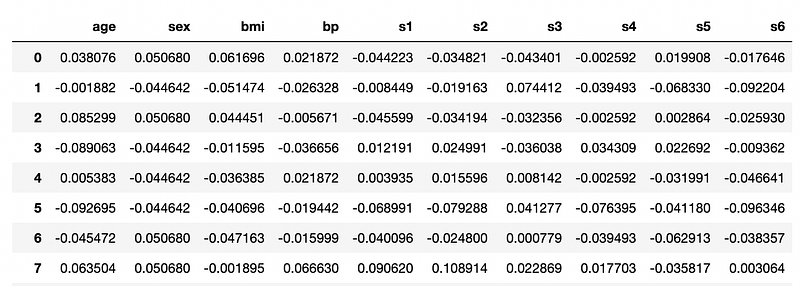
and I split it into training and test sets:
from sklearn.model_selection import train_test_splitX_train, X_test, y_train, y_test = train_test_split(X, y, test_size=0.33, random_state=42)The objective of this scenario is to calculate the blood glucose value (y value), from some input features, including body mass index (BMI), body pressure (bp), and other similar parameters. Input features are already normalized. This is a typical regression problem.
2.2 Dummy Regressor
Before applying a real Machine Learning model, I build a baseline model, i.e. Dummy Regressor, which calculates the output value as the average value of the outputs in the training set.
The Dummy Regressor can be used for comparison, i.e. check whether a Machine Learning model improves the performance with respect to it.
from sklearn.dummy import DummyRegressor
model = DummyRegressor()
model.fit(X_train, y_train)
I calculate the MSE for the model:
y_pred = model.predict(X_test)
print("Mean squared error: %.2f" % mean_squared_error(y_test, y_pred))
the output is 5755.47.
Now, I can calculate the SHAP value for this basic model. I build a generic Explainer with the model and the training set, and then I calculate the SHAP values on a dataset, which can be different from the training set. In my example, I calculate the SHAP values for the training set.
import shapexplainer = shap.Explainer(model.predict, X_train)
shap_values = explainer(X_train)Note that the Explainer may receive as input the model itself or the model.predict function, depending on the model type.
The shap library provides different functions to plot the SHAP values, including the following ones:
summary_plot()— show the contribution of each feature to the SHAP values;scatter()— show the scatter plot of SHAP values versus every input feature;plots.force()— interactive plot, for all the datasets;plots.waterfall()— show how the SHAP value is built for a single data.
Before calling the previous functions, the following command must be run:
shap.initjs()Firstly, I draw the scatter plot:
shap.plots.scatter(shap_values, color=shap_values)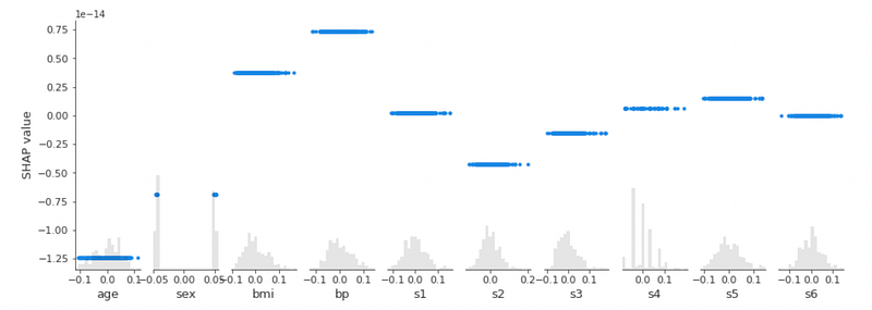
The previous graph shows what was expected: in a Dummy model, each feature gives a constant contribution to the SHAP value.
Now, I draw the summary plot:
shap.summary_plot(shap_values, X_train, plot_type='bar')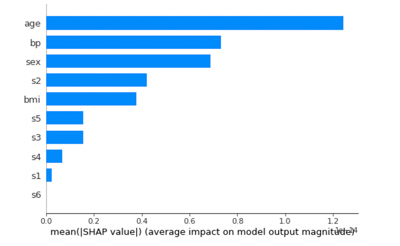
It is interesting to note how in a dummy model, the most influential factor is age.
Finally, I plot the force() plot. The following figure is static, but if you plot in a notebook, it is interactive:
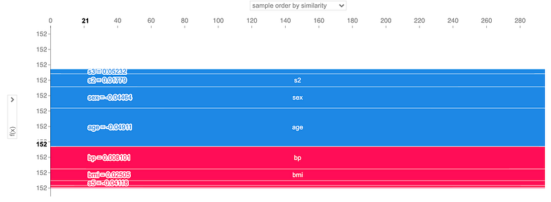
Obviously, for every sample in the dataset (x-axis) each feature gives the same contribution to the predicted value (y-axis).
2.3 Linear Regressor
The Dummy Regressor does not seem the best model, because it achieves MSE = 5755.47. I try a Linear Regressor, in the hope that it achieves a better performance.
from sklearn.linear_model import LinearRegression
model = LinearRegression()model.fit(X_train, y_train)
y_pred = model.predict(X_test)
print("Mean squared error: %.2f" % mean_squared_error(y_test, y_pred))The Linear Regressor has MSE = 2817.80, which is better than the dummy model.
I build the Explainer, which receives the model as input:
import shap
explainer = shap.Explainer(model, X_train)
shap_values = explainer(X_train)
Now, I plot the summary plot:
shap.summary_plot(shap_values, X_train, plot_type='bar')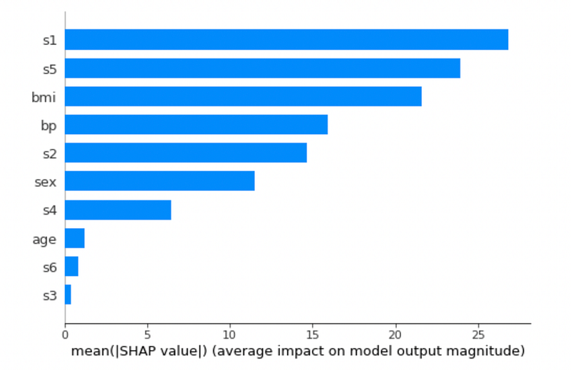
In this case, the most influential feature is s1 (in the Dummy model, the most influential feature was age). The summary plot can be also drawn without specifying the plot_type parameter:
shap.summary_plot(shap_values, X_train)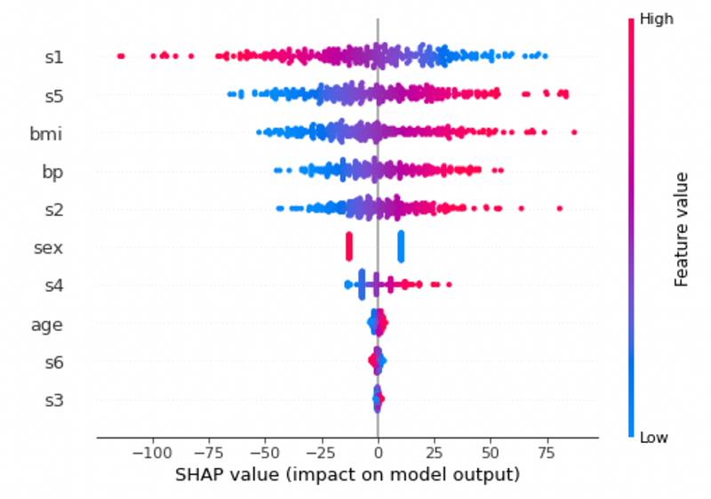
The previous graph shows the contribution of each input feature to the SHAP value. Note that SHAP values less than -75 are determined only by s1.
I draw the waterfall graph for sample 0 in the training set:
shap.plots.waterfall(shap_values[2])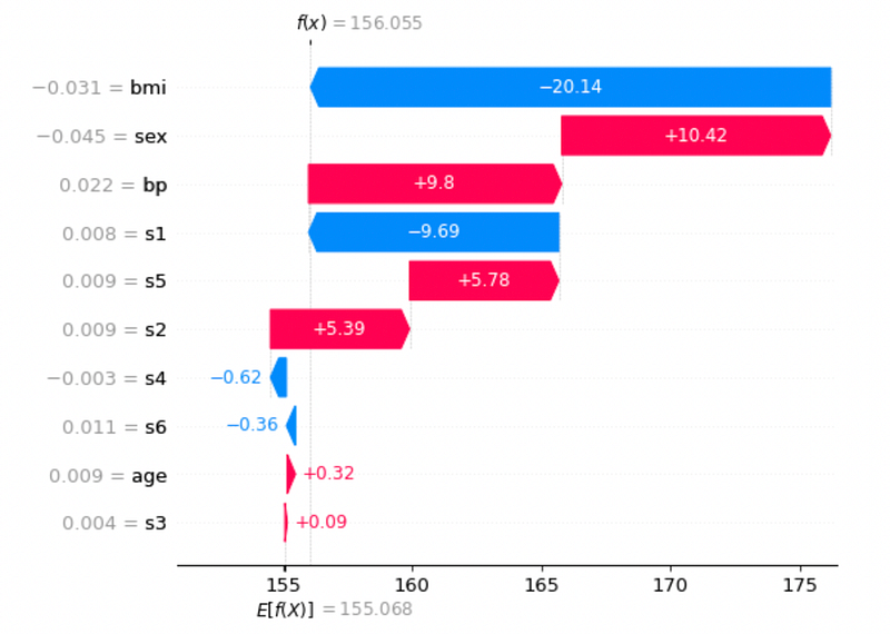
The previous graph shows how the final prediction f(x) is built from the baseline value E[f(x)]. Red bars give a positive contribution, blue ones give a negative contribution.
I can show the previous graph for all the samples, through force() graph:
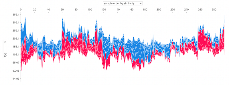
With respect to the same graph built for the Dummy Regressor (that is flat), for the Linear Regressor, the contribution of every feature to the final outcome depends on the single sample.
Finally, I plot the scatter plot:
shap.plots.scatter(shap_values, color=shap_values)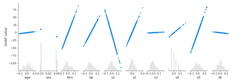
2.4 SGD Regressor
Finally, I implement a Stochastic Gradient Descent Regressor. I exploit a Grid Search with Cross Validation to tune model:
from sklearn.model_selection import GridSearchCV
parameters = {
    'penalty' : ('l2', 'l1', 'elasticnet')
}
model = SGDRegressor(max_iter=100000)
clf = GridSearchCV(model, parameters)
clf.fit(X_train, y_train)
I calculate MSE:
model = clf.best_estimator_y_pred = model.predict(X_test)
print("Mean squared error: %.2f" % mean_squared_error(y_test, y_pred))The model reaches a MSE = 2784.27, which is better than the previous models.
The following figure shows the summary plot:
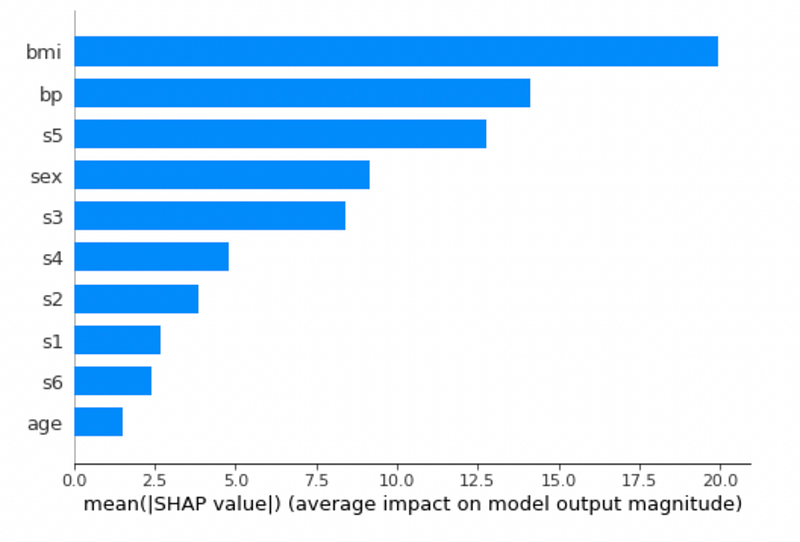
The previous graph shows that the bmi feature is the most influential parameter for a SGD classifier.
Summary
Congratulations! You have just learned how to reverse a Machine Learning model through the SHAP value! The SHAP value specifies how each feature contributes to the final predicted value.
If you have come this far to read, for me it is already a lot for today. Thanks! You can read more about me in this article.
References
- https://coderzcolumn.com/tutorials/machine-learning/shap-explain-machine-learning-model-predictions-using-game-theoretic-approach
- https://m.mage.ai/how-to-interpret-and-explain-your-machine-learning-models-using-shap-values-471c2635b78e
- https://www.kaggle.com/dansbecker/advanced-uses-of-shap-values
- https://shap.readthedocs.io/en/latest/example_notebooks/overviews/An%20introduction%20to%20explainable%20AI%20with%20Shapley%20values.html


