CLASSIFICATION TASK

A Machine Learning Approach To Credit Risk Assessment

Predicting loan defaults and their probability

1. Introduction

Credit default risk is simply known as the possibility of a loss for a lender due to a borrower’s failure to repay a loan. Credit analysts are typically responsible for assessing this risk by thoroughly analyzing a borrower’s capability to repay a loan — but long gone are the days of credit analysts, it’s the machine learning age! Machine learning algorithms have a lot to offer to the world of credit risk assessment due to their unparalleled predictive power and speed. In this article, we will be utilizing machine learning’s power to predict whether a borrower will default on a loan or not and to predict their probability of default. Let’s get started.

2. Dataset

The dataset we’re using can be found on Kaggle and it contains data for 32,581 borrowers and 11 variables related to each borrower. Let’s have a look at what those variables are:

• Age — numerical variable; age in years
• Income — numerical variable; annual income in dollars
• Home status — categorical variable; “rent”, “mortgage” or “own”
• Employment length — numerical variable; employment length in years
• Loan intent — categorical variable; “education”, “medical”, “venture”, “home improvement”, “personal” or “debt consolidation”
• Loan amount — numerical variable; loan amount in dollars
• Loan grade — categorical variable; “A”, “B”, “C”, “D”, “E”, “F” or “G”
• Interest rate — numerical variable; interest rate in percentage
• Loan to income ratio — numerical variable; between 0 and 1
• Historical default — binary, categorical variable; “Y” or “N”
• Loan status — binary, numerical variable; 0 (no default) or 1 (default) → this is going to be our target variable

Now that we know what kind of variables we’re dealing with here, let’s get to the nitty-gritty of things.

3. Data exploration and preprocessing

First, let’s go ahead and check for missing values in our dataset.

#Checking for missing values
data.isnull().sum()

Age                       0 
Income                    0 
Home_Status               0 
Employment_Length       895 
Loan_Intent               0 
loan_Grade                0 
Loan_Amount               0 
Interest_Rate          3116 
Loan_Status               0 
loan_percent_income       0 
Historical_Default        0 
dtype: int64

We can see that employment length and interest rate both have missing values. Given that the missing values represent a small percentage of the dataset, we will remove the rows that contain missing values.

#Dropping missing values
data = data.dropna(axis=0)

Next, we will look for outliers in our dataset so we can remedy them accordingly. We will do this using the describe() method which is used for calculating descriptive statistics. Not only will it help identify outliers, but it will also give us a better understanding of how our data is distributed. We’ll also be using a scatterplot matrix, a grid of scatterplots used to visualize bivariate relationships between combinations of variables, to visually detect outliers.

data.describe()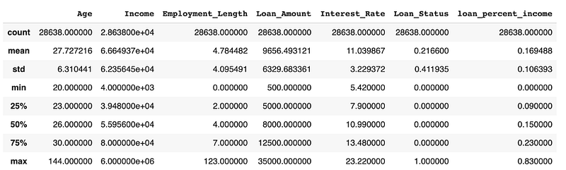

I don’t know about you but I didn’t come across that many people who have lived until the age of 144 or have been employed for 123 years. Wit aside, outliers from variables age and employment length could negatively affect our model and so should be removed. Before we do so, we’ll look for more outliers using the scatterplot matrix.

#Scatterplot matrix
fig = px.scatter_matrix(data, dimensions=
["Age","Income","Employment_Length","Loan_Amount","Interest_Rate"],
labels={col:col.replace('_', ' ') for col in data.columns},           height=900, color="Loan_Status", color_continuous_scale=px.colors.diverging.Tealrose)
fig.show()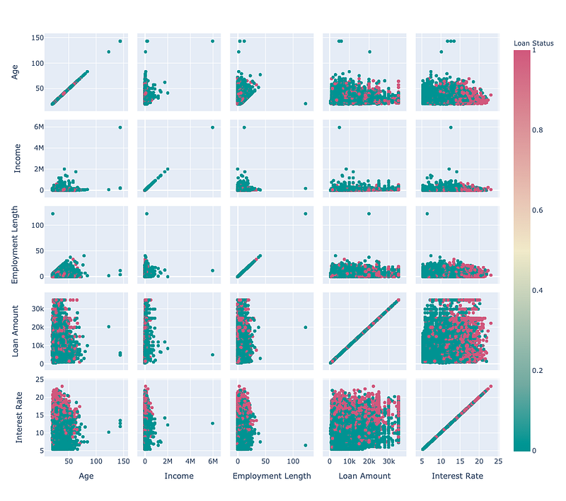

It’s now clear that income also has an outlier that needs to be removed. We’ll now remove all the outliers using the following lines of code.

#Removing outliers
data = data[data["Age"]<=100]
data = data[data["Employment_Length"]<=100]
data = data[data["Income"]<= 4000000]

Given the nature of our dataset, we’d expect that we’re dealing with an imbalanced classification problem, meaning that we have considerably more non-default cases than default cases. Using the code below, we confirm that this is indeed the case with 78.4% of our dataset containing non-default cases.

#Percentage of non-default cases
data_0 = data[data.Loan_Status == 0].Loan_Status.count() / data.Loan_Status.count()
data_0

With this in mind, we’ll now further explore how loan status is related to other variables in our dataset.

#Box plot
fig = px.box(data, x="loan_Grade", y="loan_percent_income", color="Loan_Status",
color_discrete_sequence=px.colors.qualitative.Dark24,
labels={col:col.replace('_', ' ') for col in data.columns},
category_orders={"loan_Grade":["A","B","C","D","E","F","G"]})
fig.update_layout(legend=dict(orientation="h", yanchor="bottom",
y=1.02, xanchor="right", x=1))
fig.show()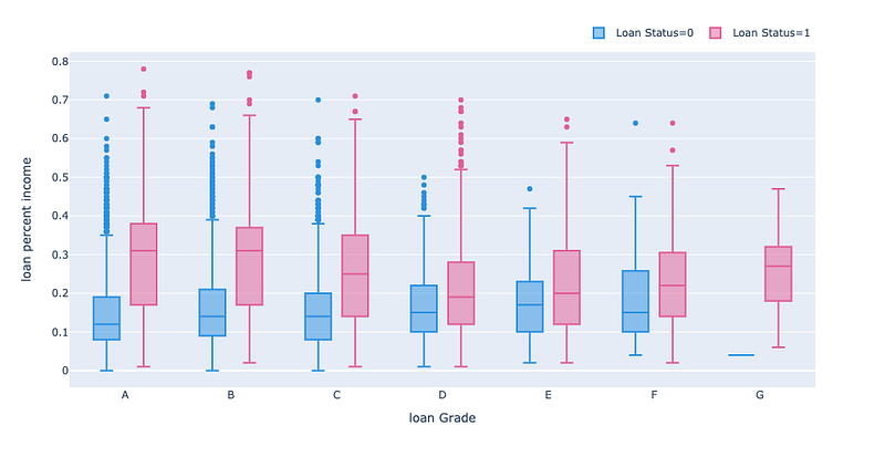

Two things quickly stand out when we look at this box plot. We can clearly see that those who don’t default have a lower loan to income ratio mean value across all loan grades; which doesn’t come as a surprise. We can also see that no borrowers with loan grade G were able to repay their loan!

Using a parallel category diagram, we can understand how different categorical variables in our dataset are related to each other and we can map out these relationships on the basis of loan status.

#Parallel category diagram
fig = px.parallel_categories(data, color_continuous_scale=px.colors.sequential.RdBu, color="Loan_Status",
dimensions=['Home_Status', 'Loan_Intent', "loan_Grade", 'Historical_Default'], labels={col:col.replace('_', ' ') for col in data.columns})
fig.show()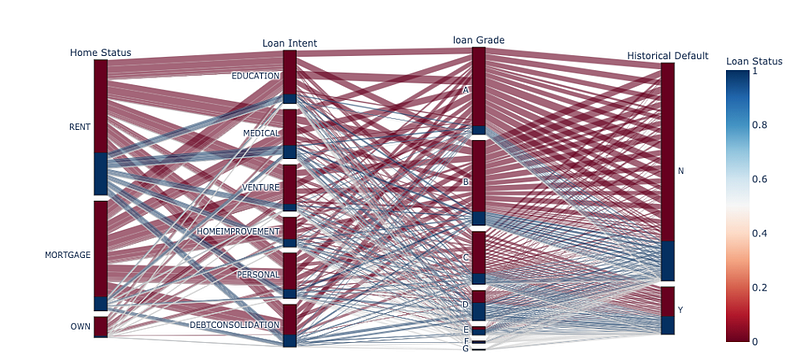

Main takeaways from the above diagram:

• Our dataset is primarily composed of borrowers who have not defaulted on a loan before;
• Loan grades “A” and “B” are the most common grades while “F” and “G” are the least common;
• Home renters defaulted more often on their loans than those with a mortgage, whereas homeowners defaulted the least;
• Borrowers took out a loan for home improvement the least and for education the most. Also, defaults were more common for loans that were taken up for covering medical expenses and debt consolidation.

Before we get into our model training, we need to make sure that all of our variables are numerical given that some of the models we’re going to use cannot operate on label data. We can simply do this using the one-hot encoding method.

#One hot encoding of categorical variables
df = pd.get_dummies(data=data,columns=['Home_Status','Loan_Intent','loan_Grade','Historical_Default'])

Now it’s time to split our dataset into a train and test split and we’ll be all ready to start building some models.

#Train and test split
Y = df['Loan_Status']
X = df.drop('Loan_Status',axis=1)
x_train, x_test, y_train, y_test = model_selection.train_test_split(X, Y, random_state=0, test_size=.20)

4. Model training and evaluation

In this section, we’ll be training and testing 3 models, namely KNN, logistic regression and XGBoost. We’ll also evaluate their performance at predicting loan defaults and their probability.

First, we’ll build the models and look at some evaluation metrics for assessing the model’s ability to predict class labels, i.e., default or no default.

def model_assess(model, name='Default'):
model.fit(x_train, y_train)
preds = model.predict(x_test)
preds_proba = model.predict_proba(x_test)
print('                   ', name, '\n',
classification_report(y_test, model.predict(x_test)))

#KNN
knn = KNeighborsClassifier(n_neighbors=151)
model_assess(knn, name='KNN')

#Logistic Regression
lg = LogisticRegression(random_state=0)
model_assess(lg, 'Logistic Regression')

#XGB
xgb = XGBClassifier(n_estimators=1000, learning_rate=0.05)model_assess(xgb, 'XGBoost')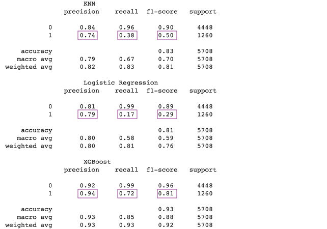

We’ve identified earlier that we are dealing with an imbalanced dataset and so we need to make sure we’re using the appropriate evaluation metrics for our case. For this reason, we’ll be looking at the common Accuracy metric with a grain of salt. To illustrate why this is the case, accuracy calculates the ratio of total truly predicted values to the total number of input samples, meaning that our model would get pretty high accuracy by predicting the majority class but would fail to capture the minority class, default, which is no bueno. This is why the evaluation metrics that we’ll be focusing on to assess the classification performance of our models are Precision, Recall and F1 score.

Firstly, Precision gives us the ratio of true positives to the total positives predicted by a classifier where positives denote default cases in our context. Given that they’re the minority class in our dataset, we can see that our models do a good job at correctly predicting those minor instances. Moreover, Recall, a.k.a true positive rate, gives us the number of true positives divided by the total number of elements that actually belong to the positive class. In our case, Recall is a more important metric as opposed to Precision given that we’re more concerned with false negatives (our model predicting that someone is not gonna default but they do) than false positives (our model predicting that someone is gonna default but they don’t). Lastly, F1 Score provides a single score to measure both Precision and Recall. Now that we know what to look for, we can clearly see that XGboost performs the best across all 3 metrics. Although it scored better on Precision as opposed to Recall, it still has a pretty good F1 score of 0.81.

We’ll now have a look at ROC which is a probability curve with False Positive Rate (FPR) on the x-axis and True Positive Rate (TPR, recall) on the y-axis. The best model should maximize the TPR to 1 and minimize FPR to 0. With this said, we can compare classifiers using the area under the curve of the ROC curve, AUC, where the higher its value, the better the model is at predicting 0s as 0s and 1s as 1s.

#ROC AUC
fig = plt.figure(figsize=(14,10))
plt.plot([0, 1], [0, 1],'r--')

#KNN
preds_proba_knn = knn.predict_proba(x_test)
probsknn = preds_proba_knn[:, 1]
fpr, tpr, thresh = metrics.roc_curve(y_test, probsknn)
aucknn = roc_auc_score(y_test, probsknn)
plt.plot(fpr, tpr, label=f'KNN, AUC = {str(round(aucknn,3))}')

#Logistic Regression
preds_proba_lg = lg.predict_proba(x_test)
probslg = preds_proba_lg[:, 1]
fpr, tpr, thresh = metrics.roc_curve(y_test, probslg)
auclg = roc_auc_score(y_test, probslg)
plt.plot(fpr, tpr, label=f'Logistic Regression, AUC = {str(round(auclg,3))}')

#XGBoost
preds_proba_xgb = xgb.predict_proba(x_test)
probsxgb = preds_proba_xgb[:, 1]
fpr, tpr, thresh = metrics.roc_curve(y_test, probsxgb)
aucxgb = roc_auc_score(y_test, probsxgb)
plt.plot(fpr, tpr, label=f'XGBoost, AUC = {str(round(aucxgb,3))}')

plt.ylabel("True Positive Rate")
plt.xlabel("False Positive Rate")
plt.title("ROC curve")
plt.rcParams['axes.titlesize'] = 18
plt.legend()
plt.show()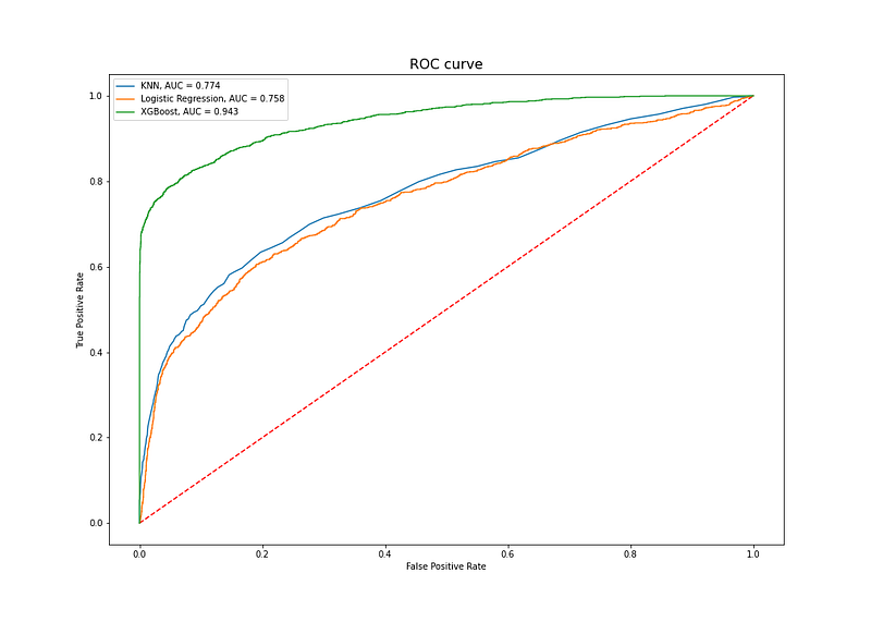

We can once again see that XGBoost performs best as it has the highest AUC and so is the best classifier in distinguishing between default and no default classes.

So far, we’ve looked at each model’s ability to predict class labels, we’ll now evaluate their performance at predicting the probability of the sample belonging to the positive class, i.e., probability of default. For this task, we’ll use a Reliability Plot and Brier Score, where the former creates a diagram of the actual probabilities versus the predicted probabilities on a test set and the latter calculates the mean squared error between predicted probabilities and their respective positive class values. Given that the Brier Score is a cost function, a lower Brier Score indicates a more accurate prediction.

#Reliability plot and Brier Score
fig = plt.figure(figsize=(14,10))
plt.plot([0, 1], [0, 1], color="black")

#KNN
knn_y, knn_x = calibration_curve(y_test, preds_proba_knn[:,1], n_bins=10, normalize=True)
loss_knn = brier_score_loss(y_test, preds_proba_knn[:,1])
plt.plot(knn_x, knn_y, marker='o', label=f'KNN, Brier score = {str(round(loss_knn,3))}')

#Logistic Regression
lg_y, lg_x = calibration_curve(y_test, preds_proba_lg[:,1], n_bins=10, normalize=True)
loss_lg = brier_score_loss(y_test, preds_proba_lg[:,1])
plt.plot(lg_x, lg_y, marker='o',label=f'Logistic Regression, Brier score = {str(round(loss_lg,3))}')

#XGBoost
preds_proba_xgb = xgb.predict_proba(x_test)
xgb_y, xgb_x = calibration_curve(y_test, preds_proba_xgb[:,1], n_bins=10, normalize=True)
loss_xgb = brier_score_loss(y_test, preds_proba_xgb[:,1])
plt.plot(xgb_x, xgb_y, marker='o', label=f'XGBoost, Brier score = {str(round(loss_xgb,3))}')

plt.ylabel("Actual probabilty")
plt.xlabel("Predicted probability")
plt.title("Reliability plot")
plt.rcParams['axes.titlesize'] = 18
plt.legend()
plt.show()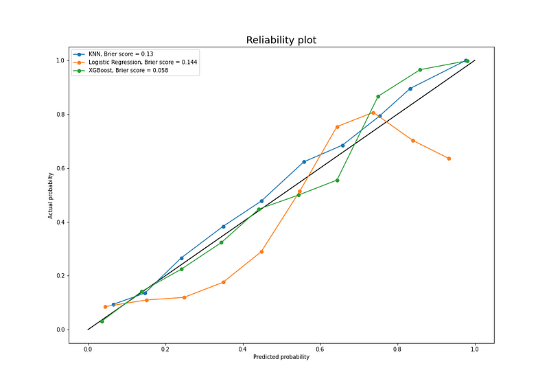

We can see from the above Brier Score that the XGBoost performs best once again, which doesn't come as a surprise by now, in comparison to other models. From this score and the plot, we conclude that our model is well-calibrated for probability prediction, meaning that predicted probabilities closely match the expected distribution of probabilities for each class, and so doesn't require further calibration.

It’s needless to say which model was chosen as our best performer at predicting class labels and the probability of default. If you've somehow skipped all previous steps and found yourself here, which you should go back and read btw, it’s XGBoost.

5. Feature Importance

Last but not least, it’s time to identify which features were most influential in predicting our target variable. For this task, we’ll be using feature importance by information gain which measures each feature’s contribution for each tree in XGBoost.

#Feature importance plot
fig, (ax1, ax2) = plt.subplots(figsize = (15, 17), ncols=1, nrows=2)
plt.subplots_adjust(left=0.125, right=0.9, bottom=0.1, top = 0.9, wspace=0, hspace = 0.5)

plot_importance(xgb, importance_type='gain', ax = ax1)
ax1.set_title('Feature Importance by Information Gain', fontsize = 18)
ax1.set_xlabel('Gain')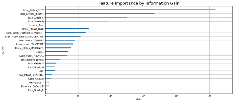

We can see from the figure above that rent as a home status, loan to income ratio and loan grade C are the top 3 most important features for predicting loan default and its probability.

Aaand that’s it!

6. Conclusion

To sum up, we’ve analyzed and pre-processed our data, trained and evaluated 3 models, namley KNN, logistic regression and XGBoost, for their ability to predict loan defaults and their probability. We used Precision, Recall, F1 and ROCAUC to evaluate the models’ performance at predicting class labels. We used these metrics in particular and discarded Accuracy given that we’re dealing with an imbalanced dataset. We also used a Reliability Plot and Brier Score to assess the calibration of our models. After having identified that XGBoost performed best on all metrics, we investigated which features were most important to our predictions using feature importance by information gain. With this said, we can round up our demonstration of how machine learning can be applied to the world of credit risk assessment.

Hope that you found this article insightful!