A Leading Fundamental Indicator for Equity Investing

Creating a Strategy on the S&P500 Using the ISM PMI in Python

Sentiment Analysis is a vast and promising field in data analytics and trading. It is a rapidly rising type of analysis that uses the current pulse and market feeling to detect what participants intend to do or what positions they are holding.

Imagine you are planning to go see a movie and you want to anticipate whether this movie will be good or not, therefore, you ask many of your friends — whom have already seen the movie — about their opinions. Assuming 75% said the movie was good, you will have a certain confidence level that you will like it because the sentiment around this movie was mostly good (ignoring tastes and preferences). The same analogy can be applied to the financial markets through many ways either quantitative or qualitative.

Sometimes, indicators will be classified as more than one type, meaning a technical indicator can also be a sentiment indicator (e.g. the On-Balance Volume). And the way we analyze can also be technical (e.g. drawing support and resistance lines) or quantitative (e.g. mean-reversion).

This article will discuss the Institute for Supply Management — Purchasing Manager’s Index and how is it used to analyze the direction of the S&P500. For this study, we will use the signal quality as a judge.

Knowledge must be accessible to everyone. This is why, from now on, a purchase of either one of my new books “Contrarian Trading Strategies in Python” or “Trend Following Strategies in Python” comes with free PDF copies of my first three books (Therefore, purchasing one of the new books gets you 4 books in total). The two new books listed above feature a lot of advanced indicators and strategies with a GitHub page. You can use the below link to purchase one of the two books (Please specify which one and make sure to include your e-mail in the note).

The ISM PMI

Sentiment Analysis is a type of predictive analytics that deal with alternative data other than the basic OHLC price structure. It is usually based on subjective polls and scores but can also be based on more quantitative measures such as expected hedges through market strength or weakness.

The Institute for Supply Management provides a monthly survey called the Purchasing Manager’s Index abbreviated to PMI, which is based on questions asked to 400 representatives of industrial companies about the current and future trend of their different activities. It is composed of 5 components that can also be analyzed individually:

• New orders — 30% weight.
• Production — 25% weight.
• Employment — 20% weight.
• Supplier Deliveries — 15% weight.
• Inventories — 10% weight.

Typically, we interpret the index as 50 being the neutral state of the economy (not growing and neither shrinking). A reading above 50 indicates an expansion in manufacturing and a reading below 50 indicates shrinking in manufacturing. The PMI tends to peak before the whole economy with a lead of 6–12 months, which makes it an astonishing leading indicator (more than 0.70 correlation with the US GDP).

It also tends to lead the stock markets. Historically the values of the PMI fluctuated between 30 and 60, so, they serve as warning signals of possible reversal. The idea of the analysis is to verify this information by creating a strategy that generates directional recommendations on the S&P500 using the idea of mean-reversion.

Downloading the Data & Designing the Strategy

Let us download a sample of both historical data of the ISM PMI and the S&P500 since 1970. I have spared you the grunt work and compiled both into an excel file downloadable from my GitHub below. This way we can import the data directly into the Python interpreter and analyze it.

The first part is to download the ISM_PMI.xlsx data to your computer and then go into the Python interpreter and switch the source to where the excel file is located. Now, we have to import it and structure it.

import pandas                    as pd
import matplotlib.pyplot         as plt
import numpy                     as np

# Defining Primordial Functions
def adder(Data, times):
    
    for i in range(1, times + 1):
    
        new = np.zeros((len(Data), 1), dtype = float)
        Data = np.append(Data, new, axis = 1)

return Data

def deleter(Data, index, times):
    
    for i in range(1, times + 1):
    
        Data = np.delete(Data, index, axis = 1)

return Data
   
def jump(Data, jump):
    
    Data = Data[jump:, ]
    
    return Data

def indicator_plot_double(Data, first_panel, second_panel, window = 250):

fig, ax = plt.subplots(2, figsize = (10, 5))
    
    ax[0].plot(Data[-window:, first_panel], color = 'black', linewidth = 1)
    ax[0].grid() 
     
    ax[1].plot(Data[-window:, second_panel], color = 'brown', linewidth = 1)
    ax[1].grid()
    ax[1].legend()

my_data = pd.read_excel('ISM_PMI.xlsx')

my_data = np.array(my_data)

Now, we should have an array called my_data with both the S&P500’s and the PMI’s historical data since 1970.

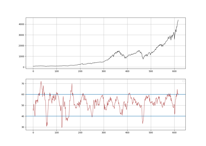
Subjectively, we can place a barrier at 40 acting as a support for the economy and a resistance at 60 acting as a break for the economy. These will be our trading triggers for buy and sell signals. Surely, some hindsight bias exists here but the idea is not to formulate a past trading strategy, rather see if the barriers will continue working in the future. Following the intuition, we can have the following trading rules:

• Long (Buy) the stock market every time the ISM PMI reaches 40.
• Short (Sell) the stock market every time the ISM PMI reaches 60.

def signal(Data, ism_pmi, buy, sell):
    
    Data = adder(Data, 2)
    
    for i in range(len(Data)):
        
        if Data[i, ism_pmi] <= 40 and Data[i - 1, buy] == 0 and Data[i - 2, buy] == 0 and Data[i - 3, buy] == 0 and Data[i - 4, buy] == 0 and Data[i - 5, buy] == 0:
            
            Data[i, buy] = 1

elif Data[i, ism_pmi] >= 60 and Data[i - 1, sell] == 0 and Data[i - 2, sell] == 0 and Data[i - 3, sell] == 0 and Data[i - 4, sell] == 0 and Data[i - 5, sell] == 0:
            
            Data[i, sell] = -1
            
    return Data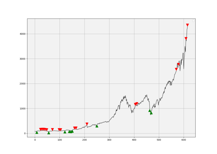

def signal_chart_ohlc_color(Data, what_bull, window = 1000):   
     
    Plottable = Data[-window:, ]
    
    fig, ax = plt.subplots(figsize = (10, 5))
    
    plt.plot(Data[-window:, 1], color = 'black', linewidth = 1)    for i in range(len(Plottable)):
        
        if Plottable[i, 2] == 1:
            
            x = i
            y = Plottable[i, 1]
        
            ax.annotate(' ', xy = (x, y), 
                        arrowprops = dict(width = 9, headlength = 11, headwidth = 11, facecolor = 'green', color = 'green'))

elif Plottable[i, 3] == -1:
            
            x = i
            y = Plottable[i, 1]
        
            ax.annotate(' ', xy = (x, y), 
                        arrowprops = dict(width = 9, headlength = -11, headwidth = -11, facecolor = 'red', color = 'red'))
    
    ax.set_facecolor((0.95, 0.95, 0.95)) 
    plt.legend() 
    plt.grid()

The code above gives us the signals shown in the chart. As a buying-the-dips indicator, the ISM PMI may require some tweaking to improve the signals. Let us evaluate this using one metric for simplicity, the signal quality.

The signal quality is a metric that resembles a fixed holding period strategy. It is simply the reaction of the market after a specified time period following the signal. Generally, when trading, we tend to use a variable period where we open the positions and close out when we get a signal on the other direction or when we get stopped out (either positively or negatively).

Sometimes, we close out at random time periods. Therefore, the signal quality is a very simple measure that assumes a fixed holding period and then checks the market level at that time point to compare it with the entry level. In other words, it measures market timing by checking the reaction of the market.

# Choosing a period
period = 21

def signal_quality(Data, closing, buy, sell, period, where):
    
    Data = adder(Data, 1)
    
    for i in range(len(Data)):
        
        try:   
            
            if Data[i, buy] == 1:
                
                Data[i + period, where] = Data[i + period, closing] - Data[i, closing]
            
            if Data[i, sell] == -1:
                
                Data[i + period, where] = Data[i, closing] - Data[i + period, closing]
                
        except IndexError:
            
             pass
         
    return Data

# Using a Window of signal Quality Check
my_data = signal_quality(my_data, 1, 2, 3, period, 4)

positives = my_data[my_data[:, 4] > 0]
negatives = my_data[my_data[:, 4] < 0]

# Calculating Signal Quality
signal_quality = len(positives) / (len(negatives) + len(positives))

print('Signal Quality = ', round(signal_quality * 100, 2), '%')
# Output: Signal Quality = 70.83%

A signal quality of 70.83% means that on 100 trades, we tend to see in 71 of the cases a profitable result if we act on it, without taking into account transaction costs. We have had 24 signals based on the conditions provided. For an indicator quoted to be a leader, the results are disappointing especially compared to the other indicators we have seen previously. However, all is not lost. Many optimization techniques can be used to improve the results:

• Add a lag factor to the S&P500 so as to see if it delivers value with historical data.
• Use another strategy based on the surpass or break of the 50 level.
• Change the barriers from 40 and 60 to 35 and 65 and see if it helps.
• See if a strategy based on exiting the barrier rather than entering the barrier is better.
• Tweak the holding period to determine the optimal reaction window.
• Change the conditions of entry and exit by including risk management and entry optimization such as closing out of a position before entering another.

If you want to see how to create all sorts of algorithms yourself, feel free to check out Lumiwealth. From algorithmic trading to blockchain and machine learning, they have hands-on detailed courses that I highly recommend.

Summary

To sum up, what I am trying to do is to simply contribute to the world of objective technical analysis which is promoting more transparent techniques and strategies that need to be back-tested before being implemented. This way, technical analysis will get rid of the bad reputation of being subjective and scientifically unfounded.

I recommend you always follow the the below steps whenever you come across a trading technique or strategy:

• Have a critical mindset and get rid of any emotions.
• Back-test it using real life simulation and conditions.
• If you find potential, try optimizing it and running a forward test.
• Always include transaction costs and any slippage simulation in your tests.
• Always include risk management and position sizing in your tests.

Finally, even after making sure of the above, stay careful and monitor the strategy because market dynamics may shift and make the strategy unprofitable.