A Journey Through Time Series, RNNs, LSTMs to the Pinnacle of Attention Mechanisms

Bridging the Gap Between Theory and Application in Predictive Modeling

#1 Introduction

Approaching Transformers and advanced language models for the first time can indeed seem formidable. My post here is to simplify this complexity into something more approachable. Here’s an outline of what I’ll cover:

Starting: I’ll begin with the basics of encoding and decoding — essential concepts at the heart of language processing.

Step further: Then, I’ll discuss the basics of traditional models such as the time series autoregression model, Recurrent Neural Networks (RNNs), and Long Short-Term Memory (LSTM) units, important for capturing how sequential data is processed.

Game changer: The focus will shift to the Transformers. These models have significantly changed the manner of natural language processing, offering new possibilities and efficiencies.

Deep Dive into Attention: I’ll learn the attention mechanism, a key component that powers Transformers and allows for their impressive capabilities in handling complex language tasks.

For readers already familiar with foundational topics such as encoding, time series analysis, and traditional neural network architectures, feel free to jump ahead to the sections focusing on Transformers and the attention mechanism.

#2 Encoding and Decoding Dynamics

‘’Machine learning can be regarded as the processes of encoding and decoding. Understanding encoding and decoding is crucial for mastering transformers and attention mechanisms, shedding light on their core role in AI models ”

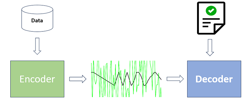
Encoding: Simplifying Data to Essentials

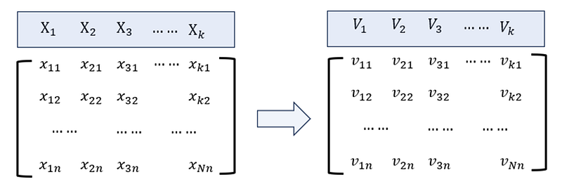
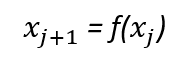
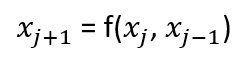
Encoding serves as an induction mechanism through which large datasets are distilled, allowing the extraction of core principles while filtering out extraneous noise. This process transforms raw data into a structured form:

Where x represents the input features within the raw data, and f(x) symbolizes the encoding transformation function. In supervised learning scenarios, the encoding operation aligns with model fitting, effectively mapping f(x) = y, where y is the target outcome. Conversely, within the realm of unsupervised learning, encoding metamorphoses into a feature transformation process, engaging in dimensionality reduction, clustering, and analogous operations found in the feed-forward or encoding phases of neural networks or transformers.

Decoding: Making Predictions and Inferences

Decoding, on the other hand, embarks on the path of inference or interpretation, applying the encoding’s outcomes to analogous data sets. In the context of machine learning and neural networks, this phase is synonymous with prediction, essentially estimating outcomes for new data instances as

The Role in Machine Learning Models

Both encoding and decoding are not standalone processes but integral components within the iterative echelons of machine learning methodologies, such as RNNs, transformers, and other iterative algorithms:

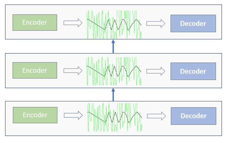
These stages recurrently feature across different layers, aiming to refine data by eradicating noise and pinpointing key influencers, thereby enhancing the model’s training efficacy and bolstering predictive accuracy.

Special Case: Autoencoders in Neural Networks

A unique application of encoding and decoding is seen in autoencoders, a neural network designed for unsupervised learning. An autoencoder consists of two parts:

· The Encoder, which compresses input data into a smaller, dense representation, focusing on the essence and ignoring the noise.

· The Decoder, which then tries to reconstruct the input from this compressed form as closely as possible to the original.

Similar Concepts in Dimensionality Reduction

This concept parallels dimensionality reduction or feature engineering in machine learning:

where techniques like principal component analysis transform raw features into principal components. Here, the transformation rule or “encoding” is defined by the loading matrix of the principal components.

In summary, encoding and decoding are fundamental to machine learning, helping models learn from data and make predictions, with applications ranging from data simplification to feature engineering and predictive modeling.

#3 Time Series Model

“Predicting future sequences in time series with the autoregressive power of attention transformers, guided by historical data trends”

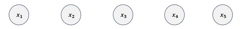
Let’s look at a straightforward question: if you see the numbers 1 to 5 in sequence, what number do you think comes next?

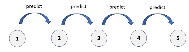
You’d probably guess the answer is 6 without much thought. But how does machine learning approach this?

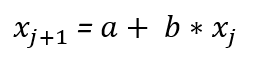
First, we use a simple model equation, assuming the model follows a linear pattern):

Using the data to express the above equation:

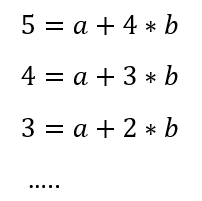
Then we find that a = 0 and b = 1

Finally, we can get the following prediction formula using linear regression (i.e. Yule method for time series autoregression):

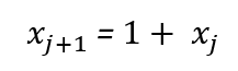
This phase of establishing the model based on the data is what we term ‘encoding,’ with our method (autoregression) being the ‘encoder’ and the derived formula the ‘encoded result.

Predicting the next number,

becomes an exercise in ‘decoding,’ utilizing our encoded model to make predictions. This straightforward example illustrates the encoding and decoding processes within machine learning clearly.

Let’s consider a different sequence: 1, 1.1, 2.3, 3.3, 5.7. What’s the next number here? This time, it’s not as straightforward.

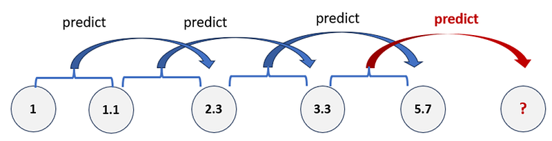
It looks like we should use the following model equation that contains two variables since the lag 1 variable does not work well in this case:

We also assume that the model is linear (linear regression):

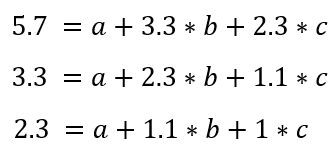
It is not so easy to guess using the brain that a = 0, b is around 1 and c is around 1. However, it is easy to get that result using machine learning, specifically linear regression.

Specifically, the above sequence seems to follow the following pattern:

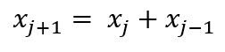
I call it a “Quasi Fibonacci Sequence” since this kind of pattern is similar to what’s called a Fibonacci sequence but with some variations — hence Quasi Fibonacci, showing the encoded relationship for this sequence.

We might prompt some reflection on our modeling choices:

· How do we know our model should be linear?

· How can we decide how many past numbers it should consider to predict the next one?

The truth is, that finding the right model can be complex. We might need to explore beyond linear models, like using polynomials or other complex functions, and decide how many past numbers to use for making accurate predictions.

#4 Recurrent Neural Networks (RNNs)

“Decoding the patterns of time with RNN models, explaining the fabric of attention transformers, blending past and present data strands”

Recurrent Neural Networks (RNNs) tackle the intricacies of forecasting by leveraging a distinct ‘Neural Network’ function, capable of modeling various relationships within time series data through its composite structure of layers and parameters:

RNNs, being nonlinear models, excel in capturing complex data relationships, setting them apart from linear models like ARIMA. Their essence lies in identifying and optimizing model parameters to accurately predict future values, a common goal shared with traditional time series models.

The key to refining RNNs is minimizing prediction errors:

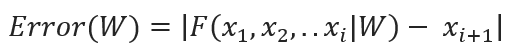
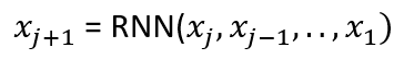
Where F() represents a broad range of possible functions, including those without explicit mathematical expressions. This step is vital for refining the model to ensure it reflects the underlying dynamics of the data accurately, RNN can be expressed as the following:

RNN Model Training: A Dual-Phase Process

Model training in RNNs prominently features gradient descent, renowned for its ability to iteratively adjust model weights W to diminish error. This process involves two main phases:

· Forward Pass: Where the model processes input data through both the encoder and decoder, generating predictions.

· Backpropagation: Utilizes the chain rule to efficiently calculate gradients and update weights across the network, enhancing the model’s learning from data and predictive accuracy.

Where Do Weight Updates Occur?

Weight updates in RNNs are not limited to the encoder. They span the entire network, including both the encoder and decoder, during the backpropagation phase following the forward pass.

Below is a Python demonstration elucidating the forward propagation process in an RNN, showcasing how input data traverses through the RNN to yield hidden state outputs:

import numpy as np
import matplotlib.pyplot as plt

# Define a simple RNN forward step function
def rnn_step(x, h_prev, Wx, Wh, b):
    """
    x: input data at the current time step.
    h_prev: hidden state from the previous time step.
    Wx: weight matrix for the input x.
    Wh: weight matrix for the hidden state.
    b: bias term.
    """
    return np.tanh(np.dot(Wx, x) + np.dot(Wh, h_prev) + b)

x = np.array([[1], [2], [5]])  # Input sequence
h0 = np.zeros((2, 1))  # Initial hidden state

# Random weights for demonstration purposes
np.random.seed(42)
Wx = np.random.randn(2, 1)
Wh = np.random.randn(2, 2)
b = np.random.randn(2, 1)
# Forward pass through RNN
h1 = rnn_step(x[0], h0, Wx, Wh, b)
h2 = rnn_step(x[1], h1, Wx, Wh, b)
h3 = rnn_step(x[2], h2, Wx, Wh, b)

# Preparing data for plotting
inputs = ['x1', 'x2', 'x3']
h_states = ['h1', 'h2', 'h3']
values = np.hstack((x.flatten(), h1.flatten(), h2.flatten(), h3.flatten()))
colors = ['blue'] * 3 + ['red'] * 3  # Adjusted to have three reds for final h states
labels = inputs + h_states  # No duplication of h_states

# Plotting
plt.figure(figsize=(8, 5))
for i, (label, value, color) in enumerate(zip(labels, values, colors), start=1):
    plt.scatter([i], [value], color=color, label=label if colors.count(color) > 1 else None)
plt.xticks(range(1, len(labels)+1), labels, rotation=45)
plt.ylabel('Value')
plt.title('RNN Forward Pass: Inputs (x) and Final Hidden States (h)')
plt.legend()
plt.grid(True)
plt.show()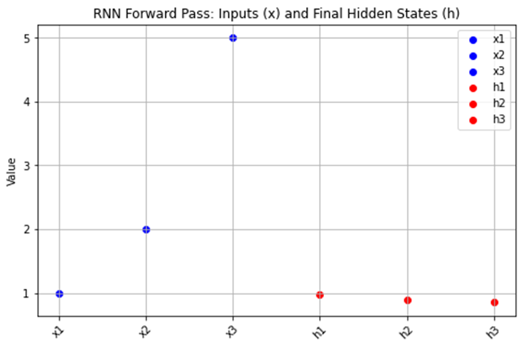

#5 Long Short-Term Memory (LSTM)

“Integrating LSTM’s memory capabilities within attention transformers to bridge intricate past data with future predictions”

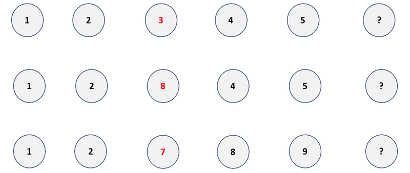
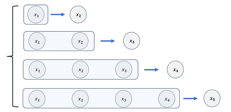
Imagine we’re trying to predict the next number in a sequence, like in these examples:

If we still use the RNN to infer the answer, the model formula is

RNNs excel with straightforward sequences but struggle with complexity, such as failing to flag an anomalous number 8 or noting the pivotal number 7 that shifts a pattern. In essence, RNNs might predict the following based on the sequences provided:

· Sequence 1: The next number increases by one

· Sequence 2: The next number is the mean of the last three

· Sequence 3: The next number is the mean of the last five.

These are attempts by RNNs to formulate rules based on the data.

The issue lies in RNNs’ basic approach to data: combining new information with past insights to form predictions. This method struggles with surprises or pattern changes, leading to confusion. Moreover, as RNNs learn and adapt, they face challenges like vanishing gradients, where updates to the model become too small to be effective, or exploding gradients, where updates are excessively large, destabilizing the learning process.

Here’s a brief explanation of these phenomena:

· RNNs linearly mix current inputs and past outputs, which can be problematic for complex or unusual sequences.

· During backpropagation, this linear method can cause:

Ø Vanishing Gradients: Too-small weight updates, impeding learning.

Ø Exploding Gradients: Too-large weight updates, causing erratic learning.

LSTMs (Long Short-Term Memory units) enhance RNNs by managing information retention and omission, improving adaptability to pattern changes and unexpected inputs.

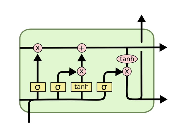
Through a unique architecture featuring input, forget, and output gates, LSTMs decide precisely what to keep, discard, and pass on, enabling precise and efficient handling of long-term dependencies in data sequences. This results in more accurate predictions for complex tasks requiring deep contextual understanding.

· Sequence 1: Continues the increment by one

· Sequence 2: Skips the outlier, maintaining the increment by one

· Sequence 3: Adapts to the new pattern, increasing by one from the new base.

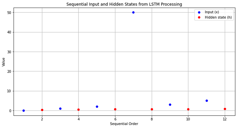
The subsequent Python code demonstrates how LSTMs process an input sequence, including an outlier 50 at x = [0, 1, 2, 50, 3, 5], to produce hidden states. This example underscores LSTMs’ ability to efficiently manage and utilize long-term data dependencies.

import numpy as np
import matplotlib.pyplot as plt

# Reusing the lstm_step function and parameters initialization from the previous example
def sigmoid(x):
    return 1 / (1 + np.exp(-x))

def lstm_step(x, h_prev, c_prev, Wf, Wi, Wc, Wo, bf, bi, bc, bo):
    f = sigmoid(np.dot(Wf, x) + bf)
    i = sigmoid(np.dot(Wi, x) + bi)
    c_tilde = np.tanh(np.dot(Wc, x) + bc)
    c_next = f * c_prev + i * c_tilde
    o = sigmoid(np.dot(Wo, x) + bo)
    h_next = o * np.tanh(c_next)
    return h_next, c_next

np.random.seed(42)  # Ensuring reproducible results
Wf, Wi, Wc, Wo = [np.random.randn(1, 1) for _ in range(4)]
bf, bi, bc, bo = [np.random.randn(1) for _ in range(4)]

x = np.array([0, 1, 2, 50, 3, 5])  # Input sequence
h_prev = np.zeros((1, 1))  # Initial hidden state
c_prev = np.zeros((1, 1))  # Initial cell state

# Containers for plot values
plot_x_values = []
plot_y_values = []
sequence_order = 1  # To keep track of x-axis values

# Processing the input sequence
for x_t in x:
    x_t_array = np.array([[x_t]])  # Making x_t compatible for matrix operations
    h_prev, c_prev = lstm_step(x_t_array, h_prev, c_prev, Wf, Wi, Wc, Wo, bf, bi, bc, bo)
    
    # Adding input x_t to the plot
    plot_x_values.append(sequence_order)
    plot_y_values.append(x_t)
    sequence_order += 1
    
    # Adding hidden state h_t to the plot
    plot_x_values.append(sequence_order)
    plot_y_values.append(h_prev.flatten()[0])
    sequence_order += 1

# Plotting
plt.figure(figsize=(12, 6))
plt.scatter(plot_x_values[::2], plot_y_values[::2], color='blue', label='Input (x)', zorder=5)
plt.scatter(plot_x_values[1::2], plot_y_values[1::2], color='red', label='Hidden state (h)', zorder=5)

plt.xlabel('Sequential Order')
plt.ylabel('Value')
plt.title('Sequential Input and Hidden States from LSTM Processing')
plt.legend()
plt.grid(True)
plt.show()

This visualization represents how LSTMs handle sequences, spotlighting their capacity to deal with outliers, as illustrated by the ability to process an anomalous input within the sequence effectively.

#6 Transformer

“Elevating the clarity of linguistic analysis beyond time series, RNN, and LSTM by sharpening focus on the symphony of words to unveil deeper linguistic contexts”

#6.1 Attention Mechanism

Imagine we’re back to the number guessing game, but with a twist, highlighting how traditional models like RNN and LSTM approach sequence processing and where Attention comes into play:

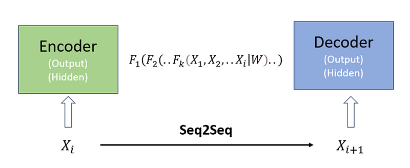
Both RNN and LSTM establish a model function using a sequence processing approach:

This ‘Seq2Seq’ approach means each current data point is connected to previous data points, forming a sequence. This is particularly useful in time series forecasting. For example, you could use such data structures and forecasting algorithms, like the auto-regression model, to predict next month’s sales for a retail store.

However, when it comes to natural language processing (NLP), both RNN and LSTM face challenges. Their training data structure tends to give more weight to recent data, causing older data to be gradually overlooked in the function f(), This can be problematic because, in language, all words — regardless of their position — can be crucial to understanding a sentence’s meaning.

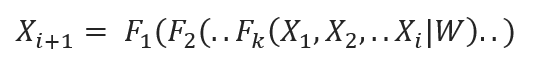
Now, consider a different approach:

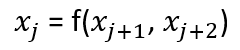
A contrasting approach involves reimagining the data relationship, not as a linear sequence but more like a network where each word or data point x can relate to any other, demonstrating the potential for words to influence each other across any distance within a document. This network-like structure addresses the inadequacies of traditional sequential models in capturing the essence of language, where the temporal order of words doesn’t always define their importance:

To enhance this process, we introduce a new data relationship structure, emblematic of what we call “Attention”, allowing the neural network to focus on contextually relevant words during translation, enhancing accuracy. Note, that attention is not a neural network but a mechanism or technique used within neural networks to improve their performance, especially in tasks involving sequences, like text processing. To realize attention, you need to construct an attention function.

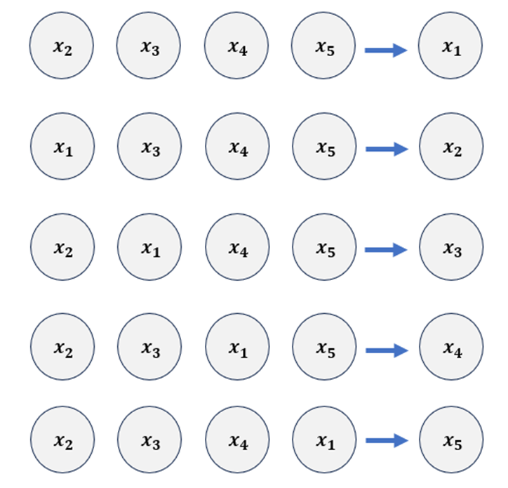
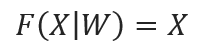
The attention applied in the transformer is called self-attention, The term “self” in self-attention signifies that the mechanism is applied within a single sequence of data, Self-attention allows each element in the sequence to interact with and be informed by every other element, enabling the model to weigh the importance of all parts of the input in the context of each specific part, self-attention is an encoder function that maps x to x itself:

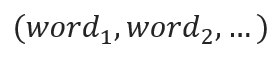
Where W is a parameter of the encoder, and X is input such as word feature (embedding vector + position encoding), but please note that the above equation is the modeling form, not the implementation or prediction formula, since X is not like the following vector joint format:

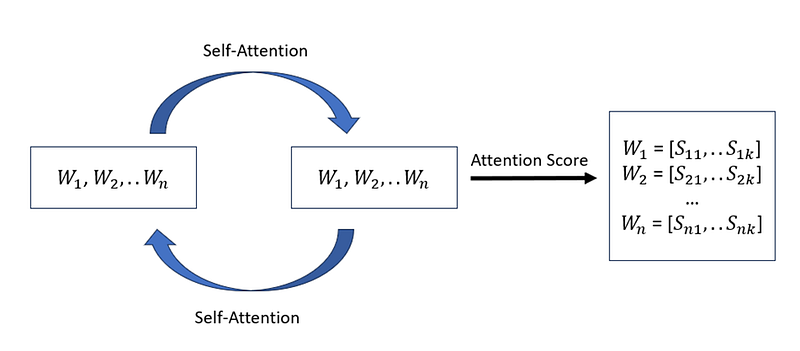
To implement self-attention (score words)

This approach highlights that self-attention assigns a distinct attention score to each word, facilitating an independent and vectorized representation of its significance within the sequence.

Understanding Self-Attention Through Optimization

The self-attention mechanism can be intuitively understood from an optimization perspective, aiming to minimize the discrepancy between the encoded representation and the input itself:

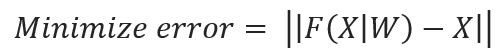
The objective is to identify an optimal set of encoder parameters W that reduces this error to a minimum. The discovery of W is achieved through the encoder’s training, employing Neural Networks’ Backpropagation. This method iteratively refines W by propagating errors backward through the entire Transformer model, encompassing both encoder and decoder components. This interconnected learning process ensures that adjustments in the encoder are informed by and contribute to the model’s overall performance, underscoring the cohesive and integrated nature of Transformer architecture learning dynamics.

#6.2 Encoding Process in Transformer

Here is a single Self-attention step (single-head attention) using a word translation job:

1. For a word sequence in a sentence,

We first express the words in a numeric form such that the computer can recognize them:

2) Model training using Neural Networks’ Back Propagation:

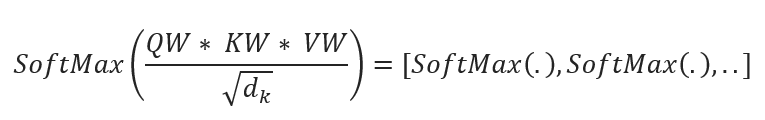
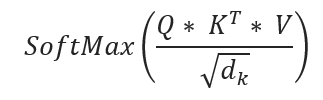
The objective is to get weight W, This is involved in the process of a specific ‘Scaled Dot-Product Attention i:

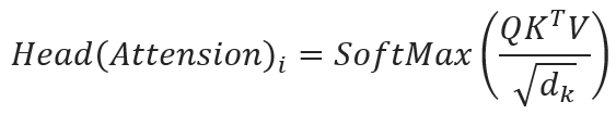
Note here the parameter W in F() is exactly the ‘Head(Attention)’, a resulting matrix that involves Query, Key, and Value weights in the above Attention calculation. Also, ‘Scaled’ means the division by the square root of the dimensionality of the key vectors), which addresses the issue of large dot products in high-dimensional spaces. this scaling ensures that the softmax function operates in a region where gradients are more meaningful and differentiation between attention weights is clearer.

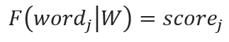
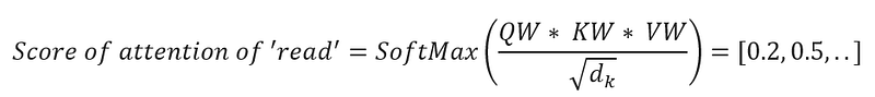
1. Calculate the score for attention for each word (word by word). The output of the self-attention for the word ‘read’ can be expressed as:

Where W is the numeric feature that expresses ‘read’, the attention score for each word is a vector, and each item of the vector will reflect how much impact this word has.

I further explain the outcome of self-attention: The output of the self-attention for each word is a new vector representation that is a weighted sum of all the original vector representations, where the weights reflect the computed relevance.

#6.3 Decoding Process in Transformer

Note, that the output of the self-attention for each word is not translation or prediction, but it tells you how to translate (output). To do this, you need the decoding process in the transformer.

The process of turning attention scores into a word or prediction during the decoding process in models like the Transformer involves several steps. These attention scores, such as

Step 1: Compute Weighted Sum

First, the attention scores are used to create a weighted sum of the value vectors V, Each element of V corresponds to an input word, and the attention scores dictate how much each of these values contributes to the output representation for “read”. Mathematically, this can be represented as:

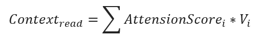
Where AttensionScore is [0.2, 0.5, ..], and V are the value vectors associated with each input word. This results in a single vector Context(‘read’) that captures the contextually relevant information for “read”.

Step 2: Generate Prediction:

The context vector Context(‘read’) is then passed through additional neural network layers, which may include:

· A feed-forward neural network within the decoder layer.

· Activation functions to introduce non-linearity.

· A final linear layer that transforms the context vector to a dimensionality that matches the size of the output vocabulary.

Step 3: Apply Softmax:

To generate a prediction from the transformed context vector, a softmax function is applied to the output of the final linear layer. The softmax function converts the logits (raw scores) into probabilities for each word in the vocabulary:

This results in a probability distribution over the entire vocabulary, where each value represents the likelihood of each vocabulary word being the next word following “read”.

Step 4: Select the Word with Highest Probability:

The word with the highest probability in the distribution becomes the model’s prediction for the next word in the sequence. For example, if “book” has the highest probability, then “book” is selected as the prediction.

#6.4 Multiple Attention Heads

The Multiple Attention Heads in transformers is a key innovation that allows the model to simultaneously attend to different parts of the input sequence from different representational spaces.

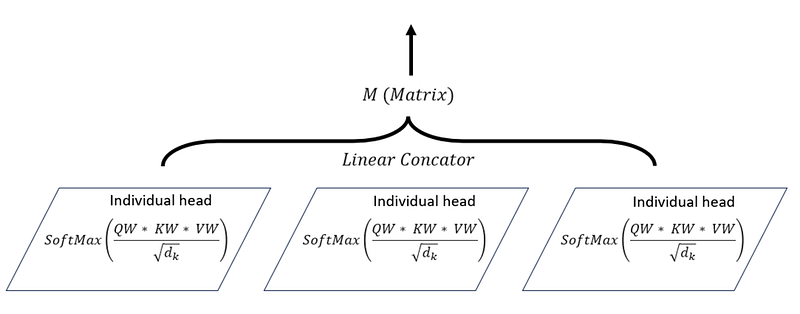
Mathematically, the outputs of the individual attention heads are then concatenated and linearly transformed to produce the final output:

Here are the benefits of Multiple Attention Heads:

· Richer Representations: By allowing the model to focus on different parts of the sequence simultaneously, multiple attention heads enable the learning of richer representations.

· Flexibility: This mechanism provides flexibility in capturing various kinds of dependencies (e.g., long-range dependencies) without increasing the computational complexity exponentially.

· Parallelization: Multiple attention heads can be computed in parallel, which significantly enhances the computational efficiency of the transformer model.

#6.5 Transformer Structure

Let’s break down a Transformer model layer by layer, starting from the input layer, focusing on a setup typically used for tasks like translation. The description follows the original “Attention is All You Need” architecture, which includes an encoder-decoder structure. Each layer in this structure builds on the outputs of the previous one to process and generate sequences.

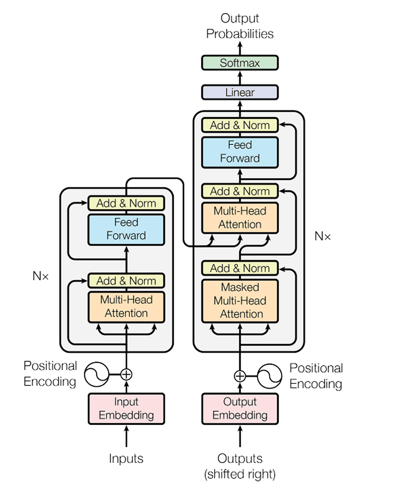
Encoder Side:

1. Input Embedding Layer:

· Word Embeddings: Converts each input word into vectors that capture semantic meanings.

· Positional Encoding: Adds information about the position of each word in the sequence to the embeddings, as Transformers do not inherently process sequences in order.

2. Encoder Layer 1-N:

Each encoder layer (commonly 6 layers are used) consists of the following subcomponents, repeated N times:

The Transformer encoder consists of a stack of identical layers (N times, where N is often 6 or more), each containing two main sub-layers:

· Multi-Head Self-Attention:

This allows each position in the encoder to attend to all positions in the previous layer of the encoder. It helps the model capture contextual relationships within the input sequence. Where each head is the attention score calculated by the Scaled Dot-Product Attention function:

· Position-wise Feed-Forward Networks (FFN): Applies a fully connected feed-forward network to each position separately and identically. This means each position flows through the same network but does so independently. In addition, The FFN comprises two stages of linear transformations, interspersed with a ReLU (Rectified Linear Unit) activation function:

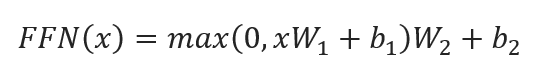
This step enhances the network’s ability to learn complex representations by applying nonlinear transformations to the attention outputs.

· Add & Norm (Residual Connection + Normalization): Each sub-layer (self-attention and feed-forward) in the encoder is followed by a residual connection and layer normalization:

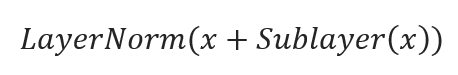
Here’s a simplified explanation:

· Sublayer(x): Applies transformations (e.g., multi-head self-attention or feed-forward networks) to inputs to enhance data structure understanding, using adjustable parameters refined during training.

· x + Sublayer(x): Adds a residual connection, combining the original input with the transformed output to ensure smooth gradient flow and address the vanishing gradient issue, enabling the construction of deeper models.

· LayerNorm(x + Sublayer(x)): Implements layer normalization on this combination, ensuring consistent activation levels across all features per sample, which leads to more stable and faster training. This approach is particularly effective for varying batch sizes, making it suitable for tasks involving sequences.

Decoder Side:

1. Output Embedding Layer:

· Word Embeddings: Similar to the input embeddings but for the target sequence.

· Positional Encoding: Added to embeddings to maintain positional information.

2. Decoder Layer 1-N:

The Transformer decoder also consists of a stack of N identical layers. However, each layer in the decoder has three main sub-layers:

· Masked Multi-Head Self-Attention: Similar to the encoder’s self-attention mechanism but with masking to prevent positions from attending to subsequent positions. This masking ensures that the predictions for position i can depend only on the known outputs at positions less than i.

· Multi-Head Attention Over Encoder’s Output: It helps the decoder focus on relevant parts of the input sequence, essentially integrating the encoder and decoder’s efforts.

· Position-wise Feed-Forward Networks: Identical to those in the encoder.

3. Final Linear Layer and Softmax:

· Linear Layer: Projects the decoder output to a much larger vector that has the size of the vocabulary.

· Softmax Layer: Converts the scores from the linear layer into probabilities, with the highest probability indicating the predicted next word in the sequence.

#6.6 Sequential Generation in Transformers

We now check how transformers construct sentences, particularly focusing on sentence translation tasks:

How Transformers Generate Sentences Step by Step: Imagine transformers as smart robots that translate sentences piece by piece. For example, when translating the sentence “I read a book,” the transformer starts by guessing the first word “read” right after seeing the beginning of a special starting sign. Then, using “read” as a clue, it moves on to predict the next word “book.” This way, each new word is guessed based on what’s already been figured out, making sure the whole sentence makes sense together.

Building Up Translations Piece by Piece: Transformers translate by taking one step at a time, using each guess to help with the next one. Starting from “read” and moving to “book,” each step relies on the previous ones to translate fit well, and sound natural.

Now we understand that transformers generate text by adding one word at a time, sticking with their initial choices for each word in the sequence. However, they can get smarter about which words to choose with the help of optimization methods such as Refinement Over Training and Beam Search. These techniques explore different ways a sentence could unfold, helping to pick the best options. This aspect falls beyond the scope of our present overview.

#7 Conclusion

This post talks about how we start with simple steps of encoding and decoding, and then move to more complex ideas like RNNs, LSTMs, and Transformers. We look closely at how Transformers pay attention to certain parts of data that matter most, changing the way computers understand language. By using Python examples, we show how these models work and how they make tasks like writing text or translating better.

We highlight how fast machine learning is growing and remind everyone of the basic ideas that keep pushing us forward. As we go on, we see how moving from simple steps to understanding complicated text with Transformers shows how much this area is changing, and there’s more exciting stuff to come.