A Guide to Volatility Trading Strategies: Long SPX vs short VIX

In this post, you will read:

• How to evaluate volatility vs. equity position trading
• How to calculate and plot the correlation of different data sets
• Use OLS and LOWESS functions for regression.

Recently, I have discussed a specific investment strategy related to volatility trading. Specifically, I have focused on shorting volatility (short vol) and compared it to long equity positions, such as those in the S&P 500 (SPX).

Understanding Short Volatility

Shorting Volatility (Short Vol) refers to strategies that profit when market volatility decreases. This is typically achieved through the use of financial instruments that track volatility indices, such as the VIX, in an inverse manner. The VIX is a measure of the market’s anticipation of future volatility over a 30-day period and is commonly known as the “fear index.”

Long equity positions, such as buying shares in the S&P 500 or an index on ETF, tend to generate gains when the market rises. Similarly, shorting volatility can exhibit similar behaviour, as volatility often decreases when markets are on the rise (and vice versa). However, as the text highlights, short volatility strategies typically have a higher mean return (average return), but they can experience significant losses during extreme market drops, also known as market tail events.

See the plot:

Each dot on the graph represents the combined performance of these two positions for a single day (see code below).

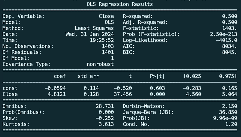
The red line on the graph represents an Ordinary Least Squares (OLS) regression analysis. OLS regression is a statistical method (part of statsmodel) that aims to minimize the differences between observed values and the values predicted by a linear function. It is a parametric approach, meaning it assumes a specific form for the relationship between variables, usually a straight line indicating a constant rate of change.

The green line represents a LOWESS (Locally Weighted Scatterplot Smoothing) regression. LOWESS is a non-parametric approach that does not assume a specific form for the relationship between the variables. Instead, it fits simple models to localized subsets of the data to build up a function that describes the deterministic part of the variation in the data, point by point. This can be particularly useful when the relationship between variables is not linear or when the data has a complex structure.

See the code:

"""
    Show correlation between SPX and VIX using OLS and LOWESS regression.
    https://quantjourney.substack.com/
    
"""
import yfinance as yf
import pandas as pd
import matplotlib.pyplot as plt
import statsmodels.api as sm

# Define the tickers
spx_ticker = '^GSPC'  # S&P 500 Index
vix_ticker = '^VIX'   # CBOE Volatility Index
# Fetch historical data
spx_data = yf.download(spx_ticker, start='2015-01-01', end='2024-01-01')
vix_data = yf.download(vix_ticker, start='2015-01-01', end='2024-01-01')
# Calculate daily returns (P&L)
spx_returns = spx_data['Close'].pct_change().dropna() * 100
vix_returns = -vix_data['Close'].pct_change().dropna() * 100
# Remove outliers
std_dev_spx = spx_returns.std()
mean_spx = spx_returns.mean()
std_dev_vix = vix_returns.std()
mean_vix = vix_returns.mean()
spx_returns = spx_returns[(spx_returns > mean_spx - 2 * std_dev_spx) & (spx_returns < mean_spx + 2 * std_dev_spx)]
vix_returns = vix_returns[(vix_returns > mean_vix - 2 * std_dev_vix) & (vix_returns < mean_vix + 2 * std_dev_vix)]
# Align indices after removing outliers
spx_returns, vix_returns = spx_returns.align(vix_returns, join='inner')
# Prepare data for OLS regression
X = sm.add_constant(spx_returns) # adding a constant
model = sm.OLS(vix_returns, X).fit()
prediction = model.predict(X)
# LOWESS regression
lowess = sm.nonparametric.lowess(vix_returns, spx_returns, frac=0.3)
# Create a scatter plot with OLS and LOWESS regression lines
plt.figure(figsize=(10, 6))
plt.scatter(spx_returns, vix_returns, alpha=0.5)
plt.plot(spx_returns, prediction, color='red', label='OLS Regression Line') # OLS Regression Line
plt.plot(lowess[:, 0], lowess[:, 1], color='green', label='LOWESS Line') # LOWESS Line
plt.title('Daily P&L: SPX vs VIX with OLS and LOWESS Regression Lines (Outliers Removed)')
plt.xlabel('SPX Daily P&L (%)')
plt.ylabel('VIX Daily P&L (%)')
plt.legend()
plt.grid(True)
plt.show()
# Print OLS regression results
print(model.summary())

You may see I have removed outliners with:

spx_returns = spx_returns[(spx_returns > mean_spx - 2 * std_dev_spx) & (spx_returns < mean_spx + 2 * std_dev_spx)]
vix_returns = vix_returns[(vix_returns > mean_vix - 2 * std_dev_vix) & (vix_returns < mean_vix + 2 * std_dev_vix)]

but with those lines, the difference is not significant.

In this context, the OLS regression line represents the average relationship between the daily P&L of the SPX and the short VIX. On the other hand, the LOWESS line offers a smoothed local fit to the data. This can be particularly helpful in understanding complex patterns or trends that may not be captured by the simpler OLS model.

The plot shows a straightforward relationship between the profit and loss (P&L) of SPX and short VIX positions. Typically, as SPX gains (or loses), the short VIX position loses (or gains). Which we may use as a trading strategy.

The summary of OLS regression:

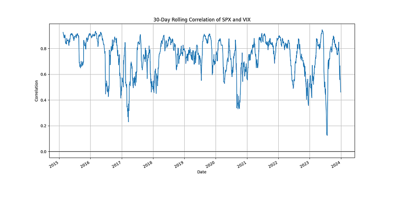
Let’s see a break over the years:

with code:

# Calculate 30-day rolling correlation
rolling_correlation = spx_returns.rolling(window=30).corr(vix_returns)

# Plot the rolling correlation
plt.figure(figsize=(14, 7))
rolling_correlation.plot(title='30-Day Rolling Correlation of SPX and VIX')
plt.ylabel('Correlation')
plt.xlabel('Date')
plt.axhline(y=0, color='black', linewidth=1)
plt.grid(True)
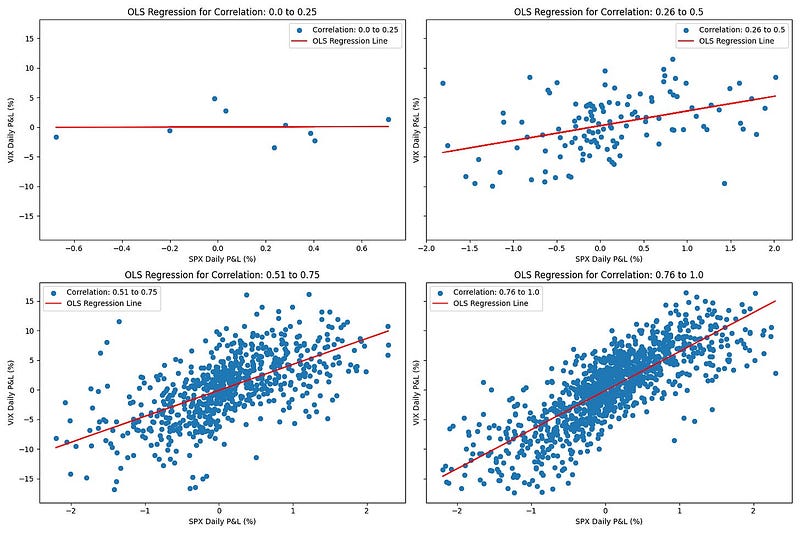
plt.show()

and as we see a correlation from 0.2 to almost 1, let’s see regression plots over the buckets where we specify them based on correlation.

with code:

# Calculate the rolling correlation
rolling_correlation = spx_returns.rolling(window=30).corr(vix_returns)

# Define the buckets of correlations
correlation_buckets = [(0.00, 0.25), (0.26, 0.50), (0.51, 0.75), (0.76, 1.00)]
# Create subplots
fig, axes = plt.subplots(2, 2, figsize=(15, 10), sharey=True)
# Iterate over the defined buckets
for i, (lower_bound, upper_bound) in enumerate(correlation_buckets):
    # Get the subset of data where the correlation falls within the current bucket
    bucket_filter = (rolling_correlation >= lower_bound) & (rolling_correlation <= upper_bound)
    bucket_spx_returns = spx_returns[bucket_filter]
    bucket_vix_returns = vix_returns[bucket_filter]
    # Prepare data for OLS regression
    X = sm.add_constant(bucket_spx_returns)  # adding a constant
    model = sm.OLS(bucket_vix_returns, X).fit()
    prediction = model.predict(X)
    # Plot
    ax = axes[i//2, i%2]
    ax.scatter(bucket_spx_returns, bucket_vix_returns, label=f'Correlation: {lower_bound} to {upper_bound}')
    ax.plot(bucket_spx_returns, prediction, color='red', label='OLS Regression Line')
    ax.set_title(f'OLS Regression for Correlation: {lower_bound} to {upper_bound}')
    ax.set_xlabel('SPX Daily P&L (%)')
    ax.set_ylabel('VIX Daily P&L (%)')
    ax.legend()
plt.tight_layout()
plt.show()

How to play this?

When you expect a surge in SPX, you can short volatility (using VIXY, UVXY, SVIX, etc. — see below). Conversely, when you anticipate the market will decline, you can take a long volatility position. The value is in the mean, also with instruments with higher exposure.

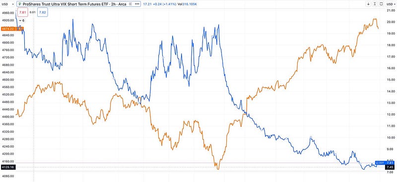
You may see the Trading View plot with SPX and UVXY for the last 6 months.

What are key Volatility Instruments?

1. UVXY: This is a 1.5X short-term ProShares ETF that provides leveraged exposure to short-term VIX futures. Its holdings are adjusted daily.
2. SVIX: This Volatility Shares ETF offers inverse exposure to short-term VIX futures with a -1.0X leverage. It rebalances daily.
3. SVXY: A ProShares ETF that provides -0.5X exposure to short-term VIX futures.
4. VXZ and VIXM: Both focus on mid-term VIX futures, with VXZ being an ETN and VIXM a ProShares ETF.

There are more, but some of those you can easily trade on most of the platforms.

Risk Management

While volatility trading can offer lucrative opportunities, it is not without risks. One of the main risks is the cost of holding positions for an extended period, which should not be overlooked.

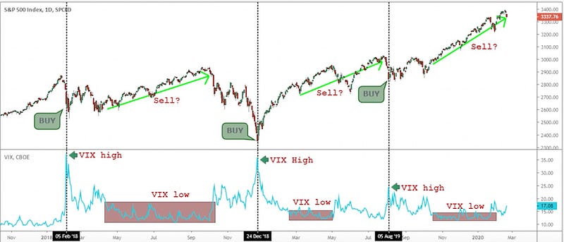
Please also note the “VIX trap”, which typically refers to a situation in the financial markets where investors are misled by a low reading of the CBOE Volatility Index (VIX). A “VIX trap” can occur when the VIX is low, suggesting that market volatility is low and conditions are stable. Investors might interpret this as a signal that the market is safe and invest more aggressively in riskier assets. However, a low VIX does not necessarily mean that the market is risk-free. If there are underlying economic or geopolitical issues that have not yet been priced into the market, or if the market is complacent, a sudden increase in volatility can catch investors off guard, leading to rapid losses.

So beware of plots like the one below — which I downloaded from the internet — as they may be misleading and give you a false sense of a good trading strategy.

— — — — — — — — — — — — — — — — — — — — — — — — — — — —