
A Gentle Introduction to Matrix Calculus
Including Applications in Machine Learning
Matrix calculus deals with derivatives and integrals of multivariate functions (functions of multiple variables). It allows us to write the partial derivatives of such functions as a vector or a matrix that can be treated as a single entity. This greatly simplifies some common mathematical operations such as finding the maximum or minimum of a multivariate function.
This article presents some of the basic definitions and rules of matrix calculus, and shows an example for applying them in machine learning.
In general, both the dependent and the independent variables of a function y = f(x) can be a scalar, a vector, or a matrix. Each different case leads to a different set of rules, or even a separate calculus. In this article I will focus on the case where x is a vector (i.e., f is a vector-valued function) and y is either a scalar or a vector.
Gradients of Scalar-Valued Functions of Vectors
First, let’s define the gradients of functions from vectors to scalars.
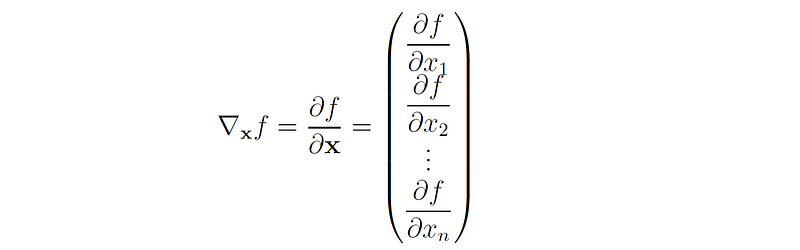
Let x = (x₁, …, xₙ)ᵗ ∈ ℝⁿ be a vector and f: ℝⁿ → ℝ a scalar function of x.
The gradient of f is defined as the vector that consists of all the partial derivatives of f with respect to the components of x:
Example 1
Given the following function from ℝ² to ℝ:

The gradient of f is:

Example 2
Let f(x) be the Euclidean norm of x squared:

Then the gradient of f is:

Proof: For each 1 ≤ i ≤ n we have:

Gradients of Vector-Valued Functions of Vectors
Next, we define the gradients of functions from vectors to vectors.
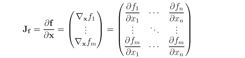
Let x = (x₁, …, xₙ)ᵗ ∈ ℝⁿ be a vector and f: ℝⁿ → ℝᵐ a vector-valued function of x.
In this case, the partial derivatives of f with respect to the components of x form the Jacobian matrix of f (denoted by J or ∇f):
Basic Rules of Derivatives of Functions of Vectors
The following rules follow directly from the properties of partial derivatives:
- Multiplication by scalar:

2. Sum of derivatives:

3. The product rule of derivatives:

4. The chain rule of derivatives:
Let f: ℝᵐ → ℝ be a scalar-valued function of a vector y ∈ ℝᵐ , where y = g(x) and g: ℝⁿ → ℝᵐ is a vector-valued function of x. Then the gradient of f with respect to x is:

Gradients of Linear Functions of Vectors
In linear functions of single variables f(x) = ax, we have the following derivation rule:

We have analogous rules for linear functions of vectors.
- Let x ∈ ℝⁿ be a vector, and f(x) = uᵗx for some known vector u ∈ ℝⁿ.
Then the gradient of f is:

Proof: For each 1 ≤ i ≤ n we have:

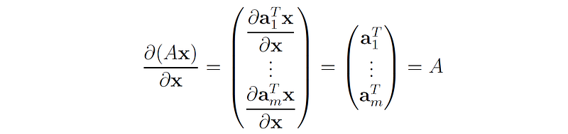
2. Let A be a matrix of size m × n , x ∈ ℝⁿ a vector, and f(x) = Ax. Then the Jacobian of f(x) is A.
Proof:
Let a₁ᵗ, …, aₘᵗ be the rows of A. Then we can write Ax as follows:

Therefore, the Jacobian of Ax is:
Gradients of Quadratic Functions of Vectors
Let A be a square matrix of size n × n , x ∈ ℝⁿ a vector, and f: ℝⁿ → ℝ the quadratic function f(x) = xᵗAx.
Then the gradient of f is:

Proof:
Let y = g(x) = Ax. Then, we can write f(x, y) = xᵗy. f is now a function of vectors x and y, where y is a function of x. Therefore, its derivative with respect to x has both a direct dependence on x and indirect dependence through the vector y = Ax.
Using the chain rule of derivatives we can write:

Note that d(f(x, y))/dx denotes the total derivative of f(x, y) with respect to both x and g(x), while ∂f(x, y)/∂x denotes the partial derivative of f(x, y) with respect to only x (keeping g(x) constant).
Then, by using the rules of gradients of linear functions we get:

As a corollary we get that if A is a symmetric matrix then:

Matrix Calculus Applications
Matrix calculus is used in derivation of:
- Kalman filters
- Regression problems in machine learning
- Gradient descent
- Expectation-maximization (EM) algorithms for Gaussian mixtures
- Deep learning theory
Example Usage in Linear Regression
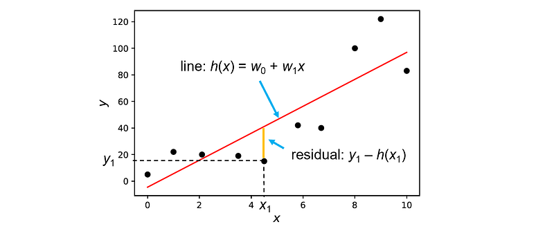
In linear regression problems, we are trying to find a linear relationship between a set of input variables x and a target variable y.
In order to learn the mapping between x and y, we are given a set of n labeled examples: D = {(x₁, y₁), (x₂, y₂), … , (xₙ, yₙ)}, where xᵢ represents the features of example i and yᵢ represents the label of that example. Based on these examples, we build a linear model of x, denoted by h(x):

Our goal is to find the parameters w of this function that will make it as close as possible to the real target y.
In ordinary least squares regression (OLS), we define a cost function that measures the sum of squared errors (residuals) between the model’s predictions h(x) and the true label y:

Our goal is to find the parameters w that will minimize J(w).
The cost function J(w) is convex under normal conditions (specifically, when the features are linearly independent), hence it has a unique global minimum. In order to find this minimum, we need to compute the gradient of J(w) with respect to each of the parameters wᵢ. Computing this gradient for each variable is very tedious. Instead, we can define the optimization problem in a matrix-vector notation.
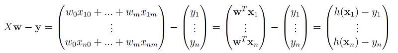
First, we define the design matrix X that contains the values of all the independent variables in the data set, including the intercept term:

The dimensions of the matrix are n × (m + 1), where n is the number of samples and m is the number of features.
In addition, we define the vector y as an n-dimensional vector that contains all the target values:

This allows us to write the least squares cost function in matrix-vector form:

Proof:
We first note that:
The dot product of a vector with itself uᵗu is just the sum of all its components squared, therefore we have:

This allows us to compute the gradient of J(w) as a function of the vector w, using the rules we have shown earlier:
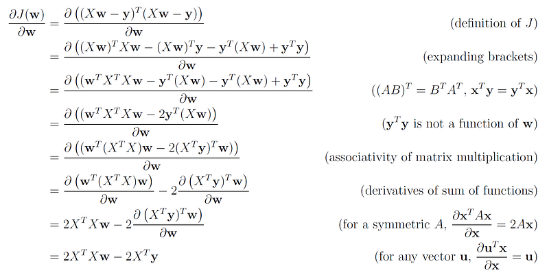
We now set this gradient to zero in order to obtain the solution for w:

Therefore, the optimal w* that minimizes the least squares cost function is:

This is known as the closed-form solution to the ordinary least squares regression problem.
You can find a numerical example for using this equation to solve a quadratic regression problem in this post.
Thanks for reading!


