A Fun Illustration of Statistical Distribution and Expectation

This neat little problem shows a great way to apply the principles of statistical distribution to calculate expected values

It’s not uncommon for data scientists and statisticians to apply statistical distributions in their work without having a basic understanding of what they are doing with these distributions. Often the distributions are deeply embedded in some code or machine learning pipeline which requires zero interaction from the user.

As many of you may know, as a mathematician and statistician, I’m a huge proponent of data scientists building a deep understanding of the mathematical concepts they work with. This will make them better data scientists and give them a greater ability to flex their methods when required.

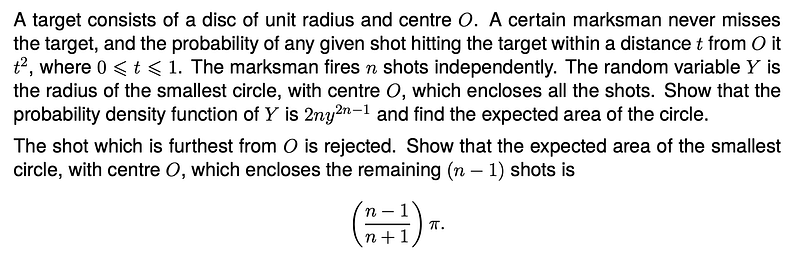
This recent problem I tackled requires a knowledge of the concept of a probability distribution function, how to construct one, and how it relates to other concepts like probability density and expected value (which many understand more intuitively as mean value). Let me start by showing you the problem.

Tackling the first part of the problem

First the problem asks us to deal with a simple situation where the marksman takes n shots and where we know that all these shots will land on the target. We are further told that the random variable Y is the radius of the smallest circle containing all those shots. Let’s try to construct some mathematical definition for Y.

Here is a diagram for a situation where the marksman has taken a few shots marked by red crosses, and where I have drawn a dotted circle with radius y to mark the minimum circle containing all the shots:

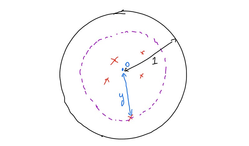
Now, if we think about it, its easy to calculate the total probability that our random variable Y is less than or equal to y. In order for Y to be less than or equal to y, we need all the n shots fired, to have landed within a distance y of O. We are told that the probability of any individual shot landing within distance t is t². So the probability of n shots landing within distance y must be:

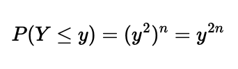
Now, we have constructed a function that tells us the total probability that our random variable Y is less than a certain value. This is known as a cumulative distribution function or cdf. If you’ve studied elementary statistics, you will know that the probability density function (pdf) of a random variable is the derivative of its cdf (or alternatively, the cdf is the integral of the pdf). Remember that the pdf of a random variable gives the probability that the random variable’s value is exactly equal to a certain value. Therefore to get the pdf P(Y = y), we just need to differentiate the cdf function above:

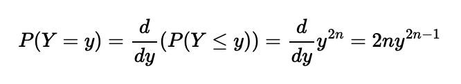
which was what we were required to show.

Now we are asked to obtain the expected value of the area of the circle that has radius defined by the random variable Y. Remember that, in the case where we have a set of discrete values for a variable, its mean represents the sum of those values times the probability of each value occurring. The expected value is simply the generalization of this concept in the case where our random variable is continuous. The formula for the expected value of a continuous random variable is

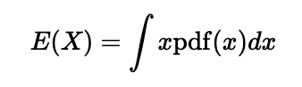
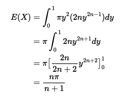
Now in this case, the random variable X is the area of the circle that has radius as our random variable Y. For any given radius y, this area is πy², and the probability of our radius y is given by our pdf function above. Therefore, noting that our radius can only take a value between 0 and 1:

Tackling the second part of the problem

In the second part we are given the complicating factor that our random variable now involves the rejection of the shot that has the furthest distance from O. Now, assuming we can work out the pdf of this new random variable — let’s call it Z — we can then just apply the same approach to finding our expected value of Z.

As before, let’s derive our cdf of Z with the aim of differentiating it to get the pdf of Z. Now for a given radius z, let’s consider how our random variable Z could be less than or equal to z. There are two possible scenarios:

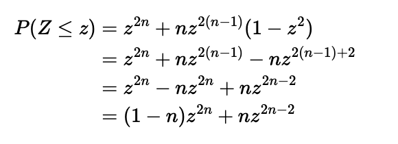
1. All n shots hit inside a radius of z. In this case, even with the furthest shot removed, all n-1 remaining shots still lie within a radius of z OR
2. All except one of the n shots hit inside a radius of z, but one did not. Given that any of the shots could be the one that does not land within the radius of z, there are n different ways that this could happen.

So we can determine our cdf of Z as

As before, we can differentiate to get the pdf of Z:

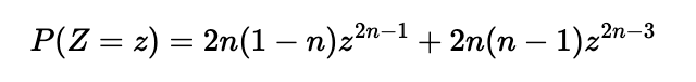
And as before we can now use this to calculate the expected value of the radius of the circle that has radius defined by the random variable Z:

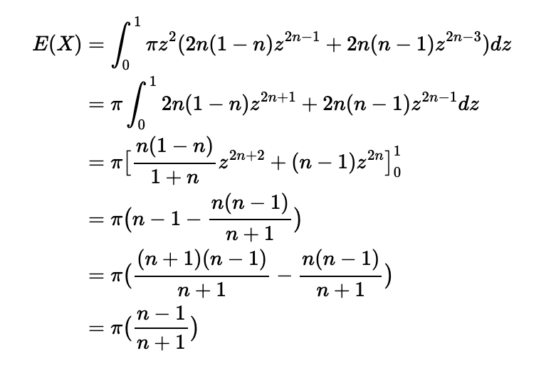
as required.

What did you think of this problem and its solution? Feel free to comment!